1  hello woRld

One of the first phrases people write across computer languages is “Hello world”. You will get to do the same in this chapter. Since we will be learning the R language, we will keep the R in the “woRld” in capital format, just for fun.

• Write basic R code using Quarto
• Get familiar with R terminology (e.g., arguments, functions, packages)
• Clone, commit, push using GitHub (optional)

1.1 Introduction to R

R is a programming language that was initially designed for statistical analysis. It is a popular language among many data scientists. If this is your first time learning a programming language, we have some good news for you. We will draw on some similarities between human languages (e.g., English) and a programming language (e.g., R). Let’s begin by looking at our first line of code in R.

print("hello woRld")

[1] "hello woRld"

You might notice a few things about this code. First, we see the code that we have written (i.e., input from us) and then, right below it, we see the R’s output. This code may seem similar to a human language. We are asking it to print “hello woRld” and in return, it prints “hello woRld”. We are great at communicating with R. It does what we are telling it to do! But before we continue telling R to do things for us, let’s learn some R vocabulary.

First, print() is what we call a function, and it prints what we tell it to print. Functions that we will see throughout this book are often represented with an action verb that tells you what the function does.

do(something)

In this case, do() is a function and something is the argument of the function. Functions can have more than one argument.

do(something, colorful)

In this case, do() is a function; something is the first argument of the function; colorful is the second argument of the function. Functions always have opening and closing parentheses.

Let’s look at something different:

my_apples <- 4

The symbols <- make up what we call an object assignment operator in R. We can think of this as the value of my_apples is set to 4. This code helps us define what the object my_apples equals to. Once defined, R will recall it from its memory as shown below.

my_apples

[1] 4

Since it is stored in memory, it can be used for different operations such as calculating the number of apples remaining after I eat one of them, as shown below.

my_apples - 1

[1] 3

R is case-sensitive which implies that lower- and upper-case lettering should be used as initially defined. For instance, R does not know the value of My_apples when writing it with a capital M. In other words, it cannot find the object My_apples since such an object (with the capital M) is not defined.

My_apples

Error: object 'My_apples' not found

When R prints out an error as output it implies that the code was not processed.

Sometimes R can also print out a warning in which case it would run the code, but it is letting us know of important constraints that might be important to consider. Lastly, R might also print out a message, which would let us know about what it has done in order to run the code.

We can use the objects we have already defined while defining newer objects as well. Let’s take a look at the following code:

n_apples <- c(7, my_apples, 13)
n_apples

[1]  7  4 13

Here we are defining a new object called n_apples, representing number of apples, using the c() function which combines three numbers: 7, my_apples, and 13. When we look at n_apples we can see that these three numbers are 7, 4, and 13 respectively since we had set my_apples to be 4 earlier.

Sometimes new learners of R wonder why the value of my_apples is 4 instead of 3 since we had already subtracted 1 from it in an earlier line of code. Even though we have indeed subtracted 1 from it, we never stored (i.e., saved or set) the value of my_apples to be 3. If we wanted to do that, we have to write:

my_apples <- my_apples - 1

On the left side of the object assignment sign <- we can see the new definition of my_apples and on the right side we have my_apples - 1 which would take the stored value of my_apples, which is 4 and subtract 1 from it. From this point onward, if we ever want to use the object my_apples, it would now be set to 3. Let’s check to make sure.

my_apples

[1] 3

We should also remind ourselves that n_apples has the old value of my_apples. In other words, making a change to my_apples would not make a change in n_apples. Code is processed in the order we run the code. We had defined n_apples before we made changes to my_apples. Let’s check to see what is in n_apples.

n_apples

[1]  7  4 13

Consider the following code and identify what the final value of red_trucks is for each case.

red_trucks <- 4

red_trucks <- 4
red_trucks + 5

red_trucks <- 4
red_trucks <- red_trucks + 5

Check footnote for answer¹

In addition to numbers, we can also combine words. For instance

names <- c("Menglin", "Gloria", "Robert")

When we ask R what the names are, we get:

names

[1] "Menglin" "Gloria"  "Robert" 

Do you notice a difference in the way we defined n_apples and names? In names we had all the elements in quotation marks. R knows a few things already including numbers (e.g. 25, 32), some functions (e.g. c()), and objects defined by us (e.g. my_age). These values and words do not need to come in quotation marks because R recognizes them. However, R has no clue about who or what Menglin is or Gloria or Robert. Thus these words are provided in quotation marks.

We call both n_apples and names vectors. Both of these vectors have three elements. Let’s get the two vectors, n_apples and names, together in a data frame:

data.frame(friend = names, apples = n_apples)

   friend apples
1 Menglin      7
2  Gloria      4
3  Robert     13

This data frame consists of three rows and two columns. Each row represents a person, and we can see their name and the number of apples they have in the corresponding columns. In the code, we need to pay close attention to the difference between friend vs. names and apples vs. n_apples. The column friend is in the data frame and it is defined by using the names vector we defined before. Similarly, the second column apples in the data frame was defined using n_apples.

If we ever want to use this data frame in the future we should store it as an object.

people <- data.frame(friend = names, apples = n_apples)

Just like any other objects, we will also refer to data frames with their name, in this case people.

people

   friend apples
1 Menglin      7
2  Gloria      4
3  Robert     13

It is always a good idea to write code first, making sure it does what you want it to do, and then store it as an object for future use.

Now that we have a data frame defined, we can select specific vectors, and values from it using the codedata_frame[row_number, column_number]. For instance, if we wanted to select Gloria, which is in the second row, and first column in the people data frame, we can write

people[2, 1]

[1] "Gloria"

We can get all of the third row by:

people[3, ]

  friend apples
3 Robert     13

We can also get all of the second column by:

people[ ,2]

[1]  7  4 13

In other words, to get all the values in a row, we specify the row number and leave the column number empty, and vice versa when wanting to select all the values in a column.

cars_passed <- data.frame(
  color = c("sedan", "truck", "van", "motorcycle"),
  number = c(10, 3, 5, 1)
)

cars_passed

       color number
1      sedan     10
2      truck      3
3        van      5
4 motorcycle      1

Consider the cars_passed data frame defined above. Identify what value(s) will be printed as output by the following code.

cars_passed[1, 1]

cars_passed[1, 2]

cars_passed[3, ]

cars_passed[3, 3]

Check footnote for answer²

At this point, reading code has been exciting. However, the best way to learn coding is by writing it. You might be wondering where you would be writing this code.

1.2 Using GUI to Write Code

You may write text in English using Microsoft Word, Google Doc, a note taking app or even in a physical notebook. Similarly in R, once you learn the R language, you can use the language in different programs (i.e., Graphical User Interfaces) such as RStudio Posit, or Microsoft Visual Studio. If you are already familiar with the command line, you can also use R on the command line. In this book, we will be using RStudio to run R code.

1.2.1 RStudio

We will discuss RStudio as an environment for coding and viewing rendered documents, but the RStudio integrated development environment has many capabilities beyond what we will cover in this book. Those additional abilities include include coding in languages other than R, such as Python, another language commonly used in data science!

When you open RStudio you will see a screen similar to the one displayed in Figure 1.1. On the left half we have the Console, and on the upper-right corner we have the Environment pane. In the lower-right corner we have the Viewer pane open, but there are many other panes such as Files and Help that we will use in this chapter and beyond.

Figure 1.1: RStudio interface

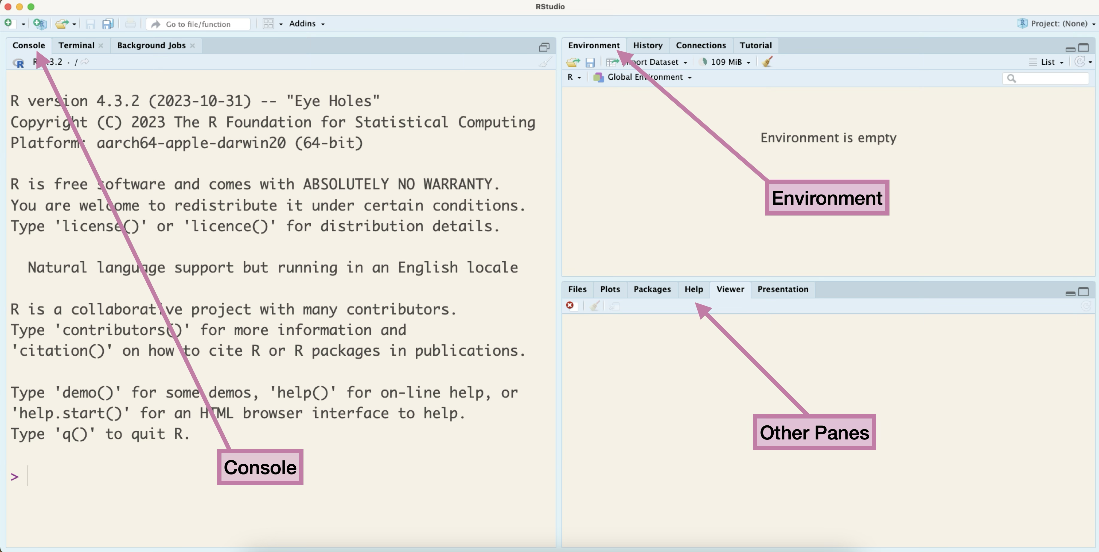
The images of RStudio in this book are from a Mac OS. If you are using a PC or another operating system, the menu or icons displayed might look a little different.

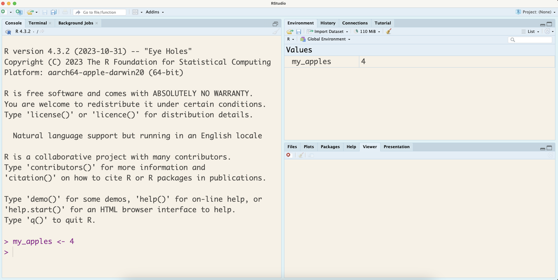
For now, we will be writing the code, in the Console section. Once you write your code, you can press Enter/return on the keyboard to run it. For instance if you write my_apples <- 4 in the Console and press Enter/return, the code is saved in the Console, but you will also notice that my_apples and its assigned value get stored in the Environment pane as seen in Figure 1.2. At this point, we would recommend you to run the rest of the code from Section 1.1.

Figure 1.2: Environment pane in the upper-right corner stores defined objects

As you begin your data science learning journey, you should not copy-paste code from this book or from the internet. Part of learning to code is building up your muscle memory. It is a good idea to type out everything you see, make typos, and learn from mistakes.

1.3 Introduction to Quarto

As a data science learner or a working data scientist, you will have to write a lot of code to analyze data. On the other hand, you will also have to write a lot of text to explain your analysis and findings to your professors, peers, boss, colleagues, or yourself. In this section, we will learn about Quarto documents which allow for writing R code³ and text at the same time. Quarto renders the R code and text to a variety of document formats including HTML, PDF, MS Word, slides, websites, and more. By the end of the book, you will be able to create some beautiful looking Quarto documents.

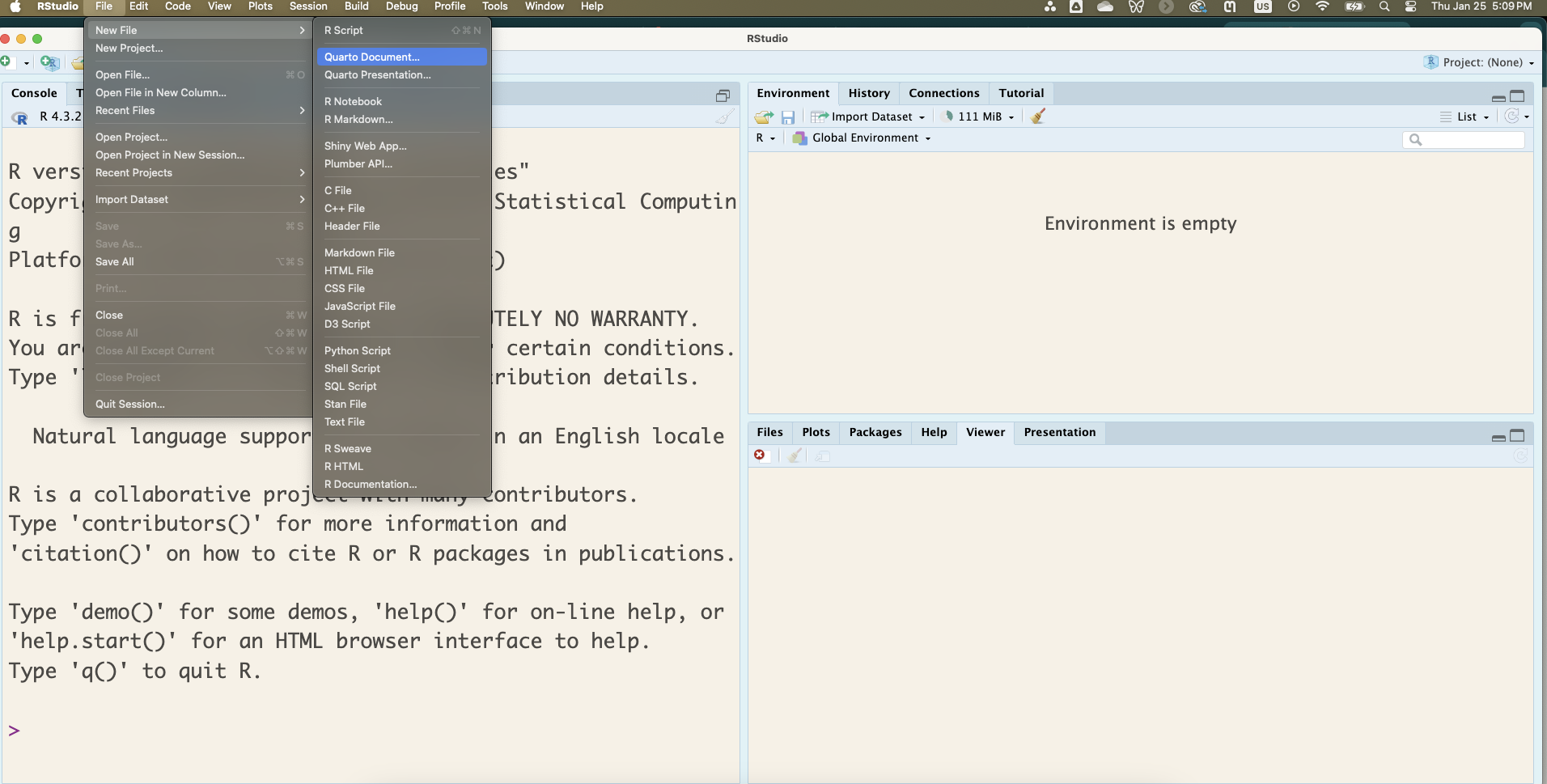
You can start a Quarto document by clicking File > New File > Quarto Document as shown in Figure 1.3.

Figure 1.3: Opening a Quarto document in RStudio

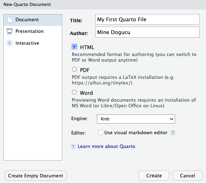
In the window that pops up, you will need to fill out the content similar to what is shown in Figure 1.4. Most importantly, make sure to set Engine to Knitr and uncheck the “Use visual markdown editor” option. When you click Create, a Quarto document will pop up in the upper left corner of your RStudio window.

Figure 1.4: New Quarto document settings

By default, RStudio will show some example text and code, which you can delete and start writing your own code. Let’s write the content as shown in Figure 1.5.

Figure 1.5: An example as a starter to Quarto as seen in the source pane

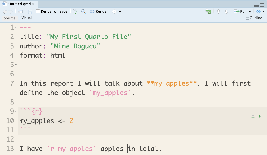
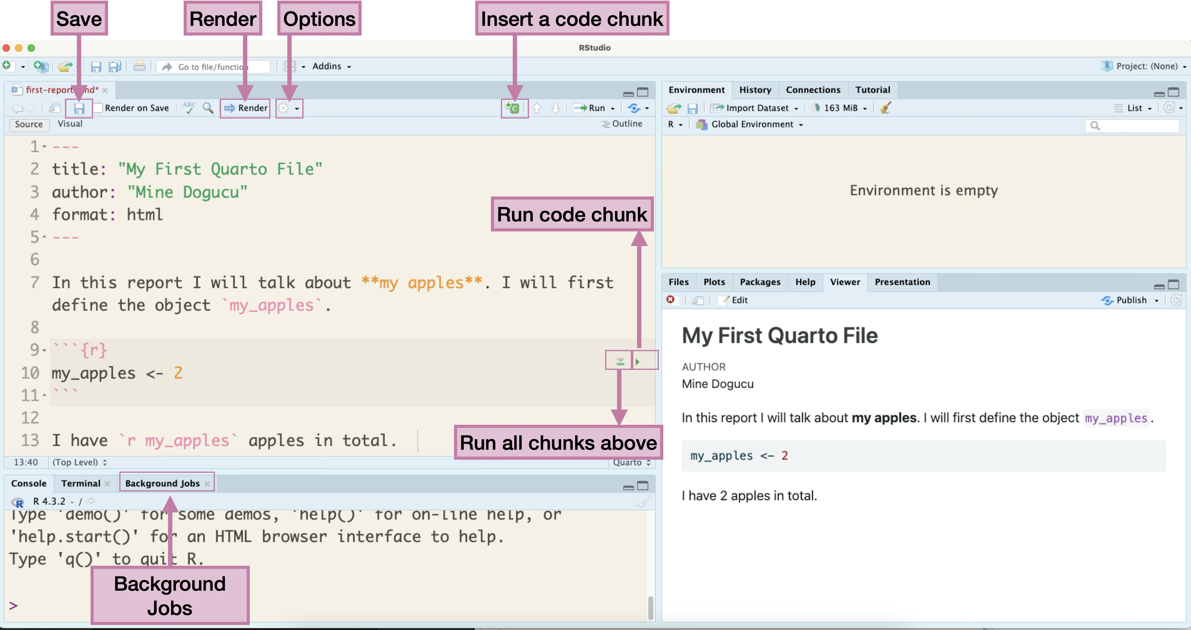
Figure 1.6 shows the full view of RStudio with certain parts highlighted. After writing the example in Figure 1.5, we can click on the Save button as highlighted in Figure 1.6. In the window that pops up, you can provide a name for your file. Make sure to choose a meaningful location where the file is saved. Do not by default save to Documents or Downloads folder. In this instance, we named the file as first-report.qmd in a folder named chapter-1, which is inside the hello-data-science folder. Depending on your operating system you may or may not see the .qmd extension of the file. This extension specifies that this is in fact a Quarto file. You may possibly have seen in the past that Microsoft Word documents, for instance, are saved as .docx at the end whether you write that or not.

Now that the first-report.qmd file is saved, we can go ahead and click on Render as highlighted in Figure 1.6. Once you render the file, an output document should appear. In Figure 1.6, the output document is displayed in the Viewer pane in the lower-right corner. To look at the different displaying choices, you can click the Options as shown in Figure 1.6 and choose to Preview in Window or Preview in Viewer Pane.

Figure 1.6: An example as a starter to Quarto, including rendered document in viewer pane

Let’s dig deeper into the contents of the Quarto document and how it is displayed in the output. Lines 2-4 of this document, are written in YAML (Yet Another Markup Language) that helps us configure some parts of the output. The title and the author lines of code set the desired title and author of the document, respectively, as shown in the output. The format option sets the format of the output file. In this instance, we chose an html file. More on this later.

In line 7, we see text written in English language with some formatting. For example, by using double asterisk (**) sign the phrase “my apples” is bolded as seen in the output⁴ We also see a backtick ( ` ) used at the beginning and end of “my_apples” which gives it a code like formatting in the output.

Lines 9 and 11 show beginning and end of an R code chunk. Anything written in a code chunk is processed as code, rather than text.

Line 13 also contains text written in English. The object my_apples is written again with backticks around it, however, the opening backtick is followed with the letter r. This is called an inline code (as opposed to a code chunk) and is processed as code, within a line of text. In fact, we can see that in the output document it is displayed as 2 since the value of it was assigned as 2 in the previous code chunk.

Lastly, we should focus on how a Quarto document is processed. Note that despite defining my_apples in the Quarto document, Figure 1.6 does not show my_apples in the Environment. After clicking the Render button, you might notice for a quick second, the Background Jobs pane getting active. Basically, a Quarto document is processed from beginning until the end. This process has nothing to do with the Console or the Environment. However, while writing code, testing out code in the Console can be convenient. In order to do that, one can send the code from the Quarto document to the Console by clicking the Run code chunk button. RStudio also conveniently provides a button to run all chunks above, which will come in handy when you have a long Quarto document with multiple code chunks.

Instead of clicking the Render button often, you can instead check the Render on Save option next to the Save button. While writing the Quarto document, you can get used to using the Ctrl+S shortcut (Cmd+S on Macs). This would save your document and then the document would get rendered automatically.

1.4 Coding for Machines and Humans

We already distinguished human languages such as English and computer languages such as R. Computer languages are processed by machines so we would like our code to be machine-readable; in other words, we would like our code not to have errors and be processed. Whether you are a student reading this book as part of your course or a self-interested reader, your code will also be read by humans possibly by your instructor, colleagues, strangers on the internet or at the very least, the code you write will be read by you! Thus, in writing code we should ensure that the code we write is not only machine-readable but also human-readable. In other words, you are communicating with your code and it is essential to follow some communication norms.

canyoureadthissentence

You probably can read the text above, but it is difficult to read it without punctuation and spaces. Just like human languages, computer languages benefit from writing with certain style rules, including spacing. However, there is not a single set of universal rules for all programming languages in all settings, as different companies or programming communities might have their own style rules. Throughout this book we will, however, follow a set of rules as described in the Tidyverse style guide (Wickham 2020).

In writing our code, we should ensure:

• Do not leave any spaces after function names (e.g., c(7, my_apples, 13)).

• Leave spaces before and after operators (e.g., <-, =).

• Put a space after a comma, not before.

• Object names are all lower case, with words separated by an underscore.

Writing human-readable code can also make it easier for others to read and reproduce your code.

1.5 R Packages

Installing R for the first time on your computer is like buying a new smart phone. It is very exciting! On one hand, new phones come with some basic functionality, you can take photos, make calls, etc. R is the same, as it comes with some built in functions, and we have in fact tried some of these functions above. On the other hand, new phones do not have all applications we may want on our phone, such as the email, social media, and news apps, among others. In this case, we would need to install apps on our phones.

Similarly, R has many packages developed by users from around the world that we can use. In order to use any functions from these packages we first need to install the packages with the code install.packages("package_name").

It is very important to install packages in the Console. If by mistake you write the code in your Quarto document, every time you render the document the package will be installed again!!! Installing a package is like installing an app on your phone. You only need to do it once. Just like apps get updated packages too get updated. From time to time you might need to update.

For example, we would like to use the say() function from the cowsay package. First, we need to install the cowsay package by writing the following code in the Console.

install.packages("cowsay")

Now that we have the cowsay package installed, let us run the say() function from this package.

say()

Error in say(): could not find function "say"

We get an error when we try to use the say() function. That is mainly because R does not know that say() is in cowsay. This is the same thing as trying to read news on the LA Times app without opening (or telling the phone to open) the LA Times app. We can solve this error in two different ways. One way can be:

1library(cowsay)
2say()

1

We are calling the cowsay package/library. From this point onward we can use any function from the cowsay package.

2

Now we are able to use the function say(). The default output of with function is an image of a cow saying Hello world!

 ______________ 
< Hello world! >
 -------------- 
      \
       \

        ^__^ 
        (oo)\ ________ 
        (__)\         )\ /\ 
             ||------w|
             ||      ||

This form of calling packages with library() function is commonly used when we use multiple functions from the same package or the same function multiple times.

We always call the packages that we need to use at the beginning of a Quarto document (after the YAML part) in the first code chunk. Someone else who reads your code should immediately see what libraries they need to use.

The second option of using a function within a package would be:

cowsay::say()

 ______________ 
< Hello world! >
 -------------- 
      \
       \

        ^__^ 
        (oo)\ ________ 
        (__)\         )\ /\ 
             ||------w|
             ||      ||

This form of calling the package is useful when using a function only once or a few times in the same document. In such cases, there would not be a need to call the whole package using library(cowsay). This option is also useful to avoid conflicts. For instance, if there was another package in R that also has a function called say() then it would be helpful to specify that we are referring to the say() function in the cowsay package.

You may also be wondering if it is possible to draw something other than a cow or have the cow say something else using the say() function. To find more information about a function and its options for the various arguments in it, we can look up the R documentation for the function in the Help pane. If you have loaded the cowsay package, then you can type ?say() in the Console and you will see the documentation pop-up in the Help pane.

Running the code ?say within the Quarto document would open a separate window with the documentation of the data. Thus, this code should not be written into the Quarto document because it will open a separate window each time the document is rendered. Hence, always use this code (i.e., ?) in the Console.

If you do not have the package loaded then you can get help by typing ??say(). Figure 1.7 shows the documentation for the say() function.

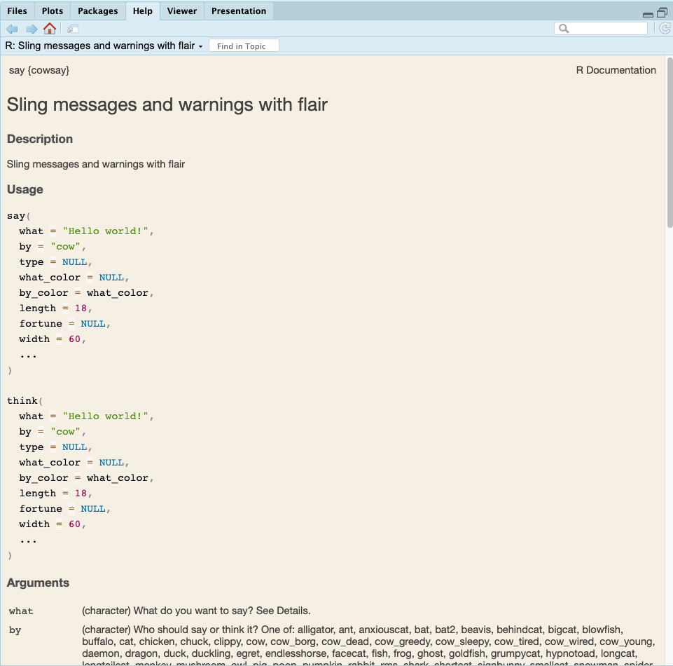
Figure 1.7: Documentation for the say() function

First of all, the documentation includes say{cowsay} at the top to indicate that this is the documentation for the say() function in the cowsay package. There are different parts to this documentation such as Description, Usage, Arguments, and Examples.

We have used the say() function without any arguments, but we can see that it actually can take many arguments as explained in the Usage section of the documentation. These arguments are then explained in the Arguments section.

The what argument is set to equal to Hello world!. Having an argument set to a specific value in the documentation indicates that it is the default value for this argument. However, it can be changed. Let’s have the cow say something different:

say(what = "I love data science already.")

 ______________________________ 
< I love data science already. >
 ------------------------------ 
      \
       \

        ^__^ 
        (oo)\ ________ 
        (__)\         )\ /\ 
             ||------w|
             ||      ||

Similarly, we can change the type of animal.

say(
  what = "I love data science already.",
  by = "cat"
)

 ______________________________ 
< I love data science already. >
 ------------------------------ 
         \
          \

            |\___/|
          ==) ^Y^ (==
            \  ^  /
             )=*=(
            /     \
            |     |
           /| | | |\
           \| | |_|/\
      jgs  //_// ___/
               \_)

Initially, reading documentation might be challenging, but it will get easier with time. Perhaps, one of the most useful sections in the documentation is the Examples section. If things are not clearly explained in the rest of the documentation, you can try to run these examples and try to create your own to figure out the capabilities of the function. Let’s try one of the examples from the documentation:

say(
  what = 'Q: What do you call a solitary shark\nA: A lone shark', 
  by = 'shark'
)

 ______________________________________________________ 
< Q: What do you call a solitary shark A: A lone shark >
 ------------------------------------------------------ 
           \
            \

              /""-._
              .       '-,
               :          '',
                ;      *     '.
                 ' *         () '.
                   \               \
                    \      _.---.._ '.
                    :  .' _.--''-''  \ ,'
        .._           '/.'             . ;
        ; `-.          ,                \'
         ;   `,         ;              ._\
          ;    \     _,-'                ''--._
          :    \_,-'                          '-._
          \ ,-'                       .          '-._
          .'         __.-'';            \...,__       '.
        .'      _,-'        \              \   ''--.,__  '\
        /    _,--' ;         \              ;           \^.}
        ;_,-' )     \  )\      )            ;
             /       \/  \_.,-'             ;
            /                              ;
         ,-'  _,-'''-.    ,-.,            ;      PFA
      ,-' _.-'        \  /    |/'-._...--'
     :--``             )/
  '

As mentioned in Section 1.4, we will be using the programming rules as described in the Tidyverse style guide. Tidyverse is not a single package but a collection of multiple packages that we will use throughout the book.

Once we install the tidyverse package, we can call the package at the beginning of our Quarto document using the library() function.

library(tidyverse)

── Attaching core tidyverse packages ──────────────────────── tidyverse 2.0.0 ──
✔ dplyr     1.1.4     ✔ readr     2.1.5
✔ forcats   1.0.1     ✔ stringr   1.5.2
✔ ggplot2   4.0.0     ✔ tibble    3.3.0
✔ lubridate 1.9.4     ✔ tidyr     1.3.1
✔ purrr     1.1.0     
── Conflicts ────────────────────────────────────────── tidyverse_conflicts() ──
✖ dplyr::filter() masks stats::filter()
✖ dplyr::lag()    masks stats::lag()
ℹ Use the conflicted package (<http://conflicted.r-lib.org/>) to force all conflicts to become errors

You might notice a few things from this output. We see which tidyverse packages (e.g., dplyr, forcats, etc.) are included when we call library(tidyverse). We also see that there are two filter functions available, one in dplyr package and one in stats package. We are notified that if we use filter() R will now be using dplyr::filter() as opposed to stats::filter(). At first R outputs might seem overwhelming. Over time, you will get better at reading the output.

Now that we have learned how to format and run code and create documents, let us talk about how we can manage our work flow with various versions of our documents.

1.6 Git and GitHub

When working on an assignment, have you ever named your files in a similar fashion to the following names: hw1, hw1_final, hw1_final2, hw1_final3, hw1_finalwithfinalimages, hw1_finalestfinal? What if we could track changes in our file with better names for each version and have only one file named hw1?

• hw1 added questions 1 through 5

• hw1 changed question 1 image

• hw1 fixed typos

In this section, we are going to learn of a system to track different versions of files. To do this, we will rely on Git and GitHub. Git is a system on our computers that allows us to track different versions of files. GitHub is a website where we can store and share different versions of the tracked files.

Throughout the book, we will use a project based workflow. You can think of a project consisting of a single file (e.g., a homework assignment can be a project) or multiple files (e.g., term project with presentation, notes, etc.,). A git repository (repo) contains all of your project’s files as well as each file’s revision history.

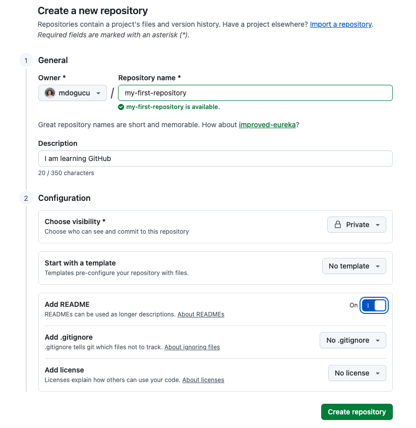
We will create our first repository while logged into GitHub by clicking the New button. Note that if you are reading this book as part of a course, your professor might have already created repos for you. Please use those repos instead. In Figure 1.8 you can see the suggested settings for your repo⁵.

Figure 1.8: Creating a new repository on GitHub

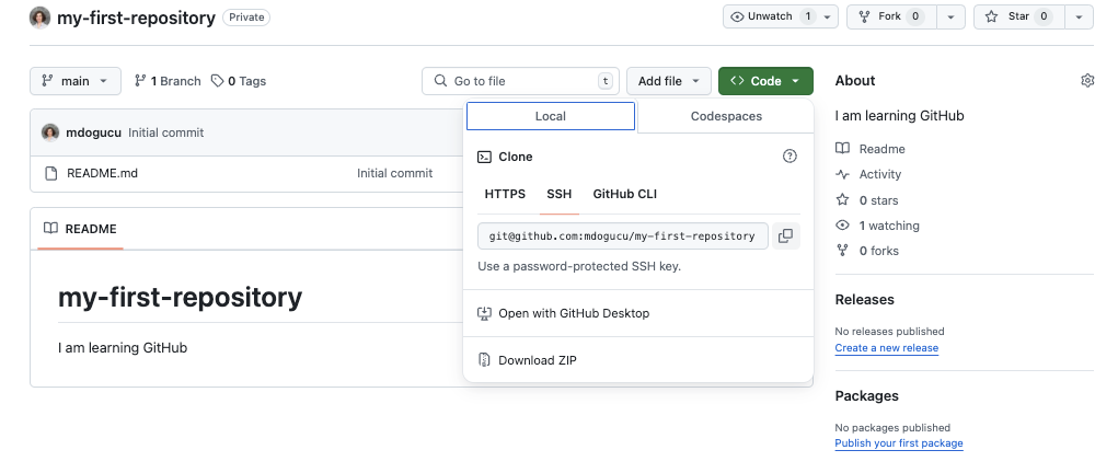
You have just created your first GitHub repo. Congratulations! It only has one file in it called README.md. Now we need to make sure we have access to this repo on our computer by clicking on Code and then SSH and we copy the link provided as seen in Figure 1.9.

Figure 1.9: Copying the repo URL

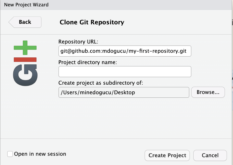
Then in RStudio’s menu bar, we click File > New Project > Version Control > Git. We should see a similar window to the one provided in Figure 1.10. You can then paste the repository URL that we just copied from GitHub and then click the Browse button to choose where you would like to store this Git project folder.

As you can see, we have chosen our Desktop; however, it is recommended for you to create a folder to accompany your learning adventure in this book.

Figure 1.10: Creating a git project in RStudio

What we have done is called cloning a repo which essentially is downloading all the elements of a repo available at that specific time. Once you clone the repo, you should notice that all the contents of the repo are shown in the Files pane. In addition to README.md file, you will see that two additional files have been created. One is .gitignore which we will delve more into in Chapter 9. The second one is my-first-repository.Rproj which is the file that makes this folder (with multiple files) be an RStudio project.

Also, you will notice that there is now a Git pane in the upper right corner in close proximity to the Environment pane that we had seen in Section 1.2.1.

Figure 1.11: Git pane in RStudio

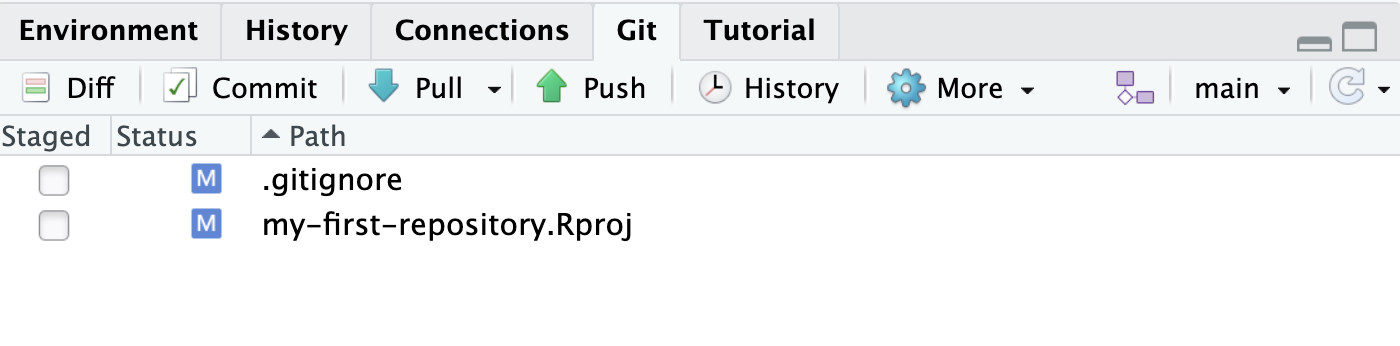
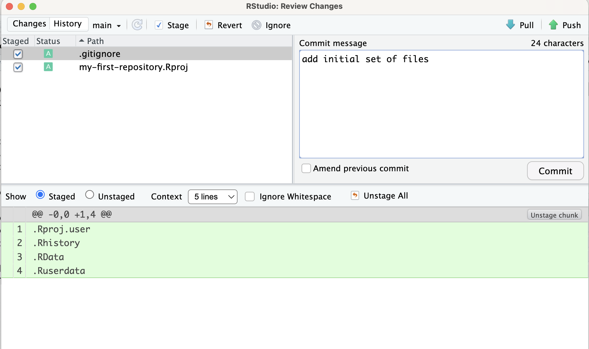
In the Git pane you can see that the two files were added with a radio button. The reason for that is because Git is watching us. The initial version of this project did not have these files, and they have newly been created. In a way, Git is alerting us “These are the changes you have made since the last version. Would you like to track them?” To do so, we can first select each of these files to be staged and press Commit. As shown in Figure 1.12, in the new window that appears, we can write in a Commit message as “add initial set of files” to describe what the new changes are and press Commit. After you commit, you might see a message reading, “Your branch is ahead of ‘origin/main’ by 1 commit”.

Figure 1.12: Commit using RStudio

Let’s step back and think about what we are doing. Once you make changes to your repo (e.g. take notes as you are reading the book) you can store the changes in the Git repository with a commit. In this instance, we made a commit which stored the two new files in our Git repo. So now we have two commits, the initial commit with just the README.md file and the second commit with README.md, .gitignore, and my-first-repository.Rproj files. We distinguish the changes from one commit to the next. We can always go back in commit history if we want to see the set of files from that specific time in the Git repository. This is especially useful, if you want to go back to an earlier solution that you have committed for a homework assignment.

Commit is local though, in other words, when we commit, we are committing to the Git project on our computer. The message “Your branch is ahead of ‘origin/main’ by 1 commit” is telling us that we have made a commit on the Git system on our computer but these changes have not been reflected on the repo stored on GitHub. In fact, if you go to the repo on GitHub you would not be able to see .gitignore and my-first-repository.Rproj files.

Let’s try clicking the Push button. You should now be able to see the changes “pushed” to GitHub. When you check the GitHub repo, you should see the two new files appear. Make sure to refresh the page if you don’t see them. We can consider pushing equivalent to uploading.

Let’s work on one more commit together. Open the README.md by finding it in the Files pane. The first line of the file is automatically set to # my-first-repository and let’s change that to # My First Repository. Save the file, click Commit, write the commit message: “add a title”, click commit, and then push.

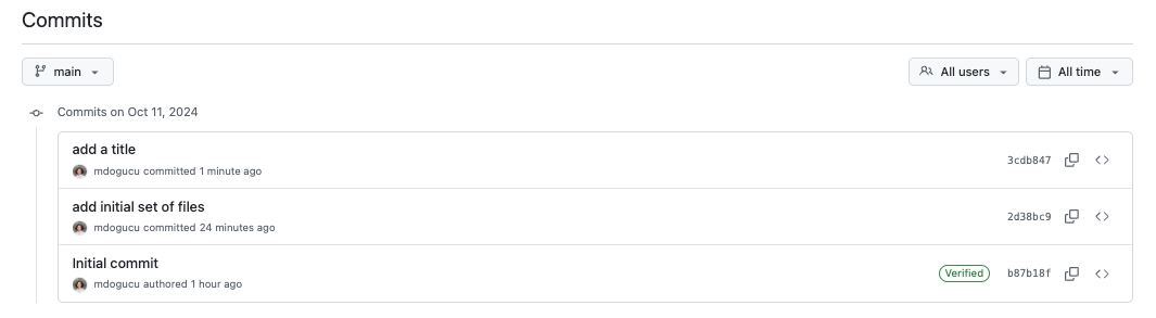
When you refresh the GitHub repo you should see the title appear the way you wrote it. In addition, you will now see the repo showing “3 commits”. When you click on “3 commits” you will see the commit history similar to one shown in Figure 1.13. The commit history allows us to go back in time and browse files at the stage that they were committed at an older date and time.

Figure 1.13: Commit history

Explain the Git and GitHub terms clone, commit, and push in your own words.

Check footnote for answer⁶

To make the most out of the commit history, it is important to write meaningful commit messages. Asking yourself “Why am I making this change and how am I making it?” can help improve commit messages.

Wickham, Hadley. 2020. The Tidyverse Style Guide. https://https://style.tidyverse.org/.

---

1. 1.) 4, 2.) 4, 3.) 9

2. 1.) sedan, 2.) 10, 3.) van, 5 4.) NULL which would indicate an error since there is no third column to index by.

3. It also supports other programming languages such as Python and Julia.

4. This kind of text formatting is handled by the markdown language. You can use the markdown cheat sheet for figuring out different text formatting options.

5. Note that your own username would be shown as the Owner of the repo.

6. Answers may vary. In simpler terms we can think of clone as downloading all files as an initial step. Commit is like a stamp that keep a record of state of files at that moment. Push uploads the commits to GitHub