In Chapter 1, we have been introduced to our toolkit. Now, we are able to use R language within RStudio using Quarto documents. In this chapter, we will introduce you to data and hopefully you will become friends.
Describe data frames
Define and use different types of variables
Define and use different storage types in R
Summarize variables using numbers
2.1 Data Frames
In addition to having functions, R packages can also have data stored in them. We will use the planets data from the {hellodatascience} package. We will first load the {hellodatascience} package by running the code library(hellodatascience). We will also load the tidyverse packages. Recall that tidyverse is not a single package but a collection of multiple packages that we will use throughout the book.
library(hellodatascience)library(tidyverse)
── Attaching core tidyverse packages ──────────────────────── tidyverse 2.0.0 ──
✔ dplyr     1.2.1     ✔ readr     2.2.0
✔ forcats   1.0.1     ✔ stringr   1.6.0
✔ ggplot2   4.0.3     ✔ tibble    3.3.1
✔ lubridate 1.9.5     ✔ tidyr     1.3.2
✔ purrr     1.2.2
── Conflicts ────────────────────────────────────────── tidyverse_conflicts() ──
✖ dplyr::filter() masks stats::filter()
✖ dplyr::lag()    masks stats::lag()
ℹ Use the conflicted package (<http://conflicted.r-lib.org/>) to force all conflicts to become errors
In order to load the planets data, we first use the data() function and then we can print out the whole dataset. Because we are taking baby steps in data science, it is OK to print the dataset for now. However, as we progress, we will see much larger datasets, and it will not be a good idea to print the dataset.
The planets data frame has 8 rows and 7 columns, as we can see in the first line of the output.
Because data is displayed in rows and columns, different data scientists call the planets object different names including dataset, data table, data matrix, and tibble. As we start learning data science, these differences will be trivial but the distinctions can be important in the long term.
We can also count the number of rows and columns as follows:
nrow(planets)
[1] 8
ncol(planets)
[1] 7
Each row represents an observation, which is defined as an object or individual we want to study.
An observational unit in this dataset is a planet in our solar system. For each observation we have some characteristics as reported in each of the columns. These characteristics are called variables because they vary from one observation to the next. The variables in the planets data frame are name, mass, length_of_day, mean_temp, n_moons, ring_system and surface_pressure. Be careful when counting the columns!!! R puts an index for row numbers (e.g., 1, 2, …, 8). However, the index number is not a column.
When encountering a data frame for the first time, some information can be deduced using common sense. For instance, we know Earth has 24 hours in a day, so we can assume that the length_of_day variable uses hours as the unit. However, it is harder to figure out the unit for mass on the spot, unless you know the planets well! Just like functions, we can also check the documentation for a data table by writing the following code in the Console.
?planets
Checking the documentation shows us that the mass variable has a unit \(10^{24} \text{ kg}\) which is read as septillion kilograms.
Now, let us learn how we can further explore the data set.
2.2 Getting to Know Data
Consider yourself working for Spotify. Can you imagine how many rows of data there must be in each data frame? Instead of printing the whole data frame, we need to rely on a few functions to help us get some idea about the data frame.
You can start exploring the data frame using the head() and tail() functions to show the first and the last six rows of the data frame, respectively.
# A tibble: 6 × 7
  name        mass length_of_day mean_temp n_moons ring_system surface_pressure
  <chr>      <dbl>         <dbl> <fct>       <int> <lgl>                  <dbl>
1 Earth      5.97           24   positive        1 FALSE                   1
2 Mars       0.642          24.7 negative        2 FALSE                   0.01
3 Jupiter 1898               9.9 negative       95 TRUE                   NA
4 Saturn   568              10.7 negative      146 TRUE                   NA
5 Uranus    86.8            17.2 negative       28 TRUE                   NA
6 Neptune  102              16.1 negative       16 TRUE                   NA
Seeing a few of the variables in the top and bottom rows of a large dataset can help us envision what the rest of the data can possibly look like.
Note that Neptune is on the eighth row in the planets data but the tail() function output shows the indexing 1 through 6 and hence Neptune is on the sixth row of the output.
The glimpse() function from the {dplyr} package can also be helpful in getting to know the data. It literally helps us take a glimpse at the data, but has a twist. Each variable is printed in a row along with few of its observations. The function glimpse() will always display all the variable names of the dataset.
The glimpse() function also prints out the number of columns and rows which can be helpful. You might also notice that next to each variable name, there is text such as chr, dbl, int or fct. More on this in Section 2.3.2.
2.3 Variable Types
Scientists love classifications!!! For instance, living things are often classified into five kingdoms: animal, plant, fungi, protista, and monera. These classifications are based on shared characteristics and can include things like cell organisation, reproduction, and movement, and so on. Not all scientists reach a consensus on this classification system. Some think there are more than five kingdoms, and some also disagree on certain species classification. Disagreements are part of science.
Sometimes disagreements in science can simply be due to one’s entry point to science. This also holds true for data science. For instance, some of you might be interested in data science simply because you like statistics and mathematics. Some of you might have ended up here because you like programming and wanted to learn R for data science. Some of you might be here because you want to make meaning of data in another scientific discipline (e.g., biology, economy, sociology, etc.). You bring different perspectives from your different disciplines to data science. You will see that, for different purposes and in different disciplines, variables can be classified differently or just with different names. We will clarify these differences and define the variable classification system that we will use throughout this book.
2.3.1 Variable Types in Statistics
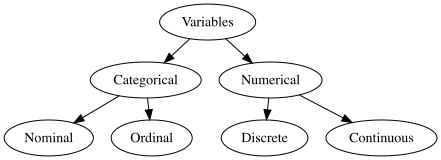
When dealing with variables, statisticians often focus on how they can analyze the variable and make meaning of it. A broad classification of variables can be considered as numerical and categorical (i.e., non-numerical). Numerical variables represent a quantity, whereas categorical variables often represent labels and not quantities, and classify observations into categories.
With numerical variables we can do arithmetic operations, such as addition or finding an average. For example, the length_of_day variable from the planets data frame is numerical, and we can talk about the average length of day for each planet. We cannot, however, talk about an average name of a planet or an average ring_system presence. Averages for those variables simply do not make sense. Thus, while length_of_day is a numerical variable, name and ring_system are categorical variables.
Variable types
A numerical variable can be turned into a categorical variable, as we can categorize observations based on a range of values. However, a categorical variable cannot be turned into a numerical variable. Thus, it is best to collect numerical information when possible and is appropriate to do so. Consider age as an example variable. If you know that somebody is 48 years old, you can categorize them as “40-49 years old”. However, if you know that someone is “40-49 years old” then you cannot know their exact age.
Numerical variables can be further classified as discrete or continuous. A discrete variable has a finite or countable number of possibilities and there are gaps between the values. For instance, n_moons is a discrete variable, as we can count the number of moons for each planet. A planet cannot possibly have 3.5 moons, 3.78 moons or 3.389 moons… On the other hand, a continuous variable can take any possible value within a specific range, and any decimal value still makes sense. For instance, the variable mass can take any value since a planet can be of any mass, and thus, it is a continuous variable.
Categorical (i.e., non-numerical) variables are further classified into two subgroups as nominal and ordinal. An ordinal variable contains categories that have a clear and meaningful order. One can often make comparisons of the ordinal groups such as “less, more, shorter, taller etc.,”. For instance, mean_temp is an ordinal variable and can be ordered from higher to lower temperature group as positive and negative. A nominal variable, on the contrary, has no order and does not represent any quantity. For instance, name is a nominal variable. Some of you might think “Well, we can order the names of planets based on distance to the Sun.” In such a case, you would be ordering based on a numerical variable distance, not the name. For nominal variables, it is up to the scientist to decide on the order of the categories, but often, these are ordered in alphabetical order.
It is also worth noting that Likert scale items such as Strongly Agree, Agree, Disagree and Strongly Disagree on surveys are very commonly used. These categories are technically ordinal, and sometimes you might see them coded as numerical by assigning numerical values such as 1, 2, 3, 4 or -2, -1, 1, 2. However, numerical operations such as taking averages of Likert scale items is not a recommended practice.
In data science we also utilize the special name of binary variables for categorical variables that represent only two groups. The word binary starts with the Latin prefix bi meaning two. Examples can include variables such as grade (pass, fail), has a pet (yes, no), medical test result (positive, negative).
In some textbooks and other readings you might come across sex or gender being treated as binary variables. However, neither of these variables are binary. You can read more on how these variables were recommended to be handled in Federal Statistical Surveys.
Variable types can be debated in different ways. For instance, consider a variable that has telephone number such as 9491234567, where the information is recorded using only numbers and no punctuation marks such as parentheses or hyphens. At data collection stage, one might argue that this variable has to be defined as numerical so that only numbers can be entered. Recall that, for numerical variables we can do certain arithmetic operations. However, calculating an average telephone number does not make sense, so someone else would argue that telephone number should be defined as categorical. Thus, when we think about variable types we have to think of them from the perspective of different scientific disciplines. While a survey statistician might be concerned about how data are entered, a computer scientist might be concerned about how data are stored on the computer, and a data analyst might be concerned about how data are analyzed. In the next subsection, we delve into classification of variables from a programming perspective in R.
Not everything represented with a number is a numerical quantity, as we saw with the telephone number example above. One important aspect of numerical quantities is that they allow us to make comparisons. For instance, based on someone’s age we can tell if they are older or younger than someone else. However, we cannot make any comparisons based on someone’s phone number.
2.3.2 Storage Types of Variables in R
Recall that the glimpse() function shows variable types such as chr, dbl, int or fct. These are the types of variables as stored in R. We can also use the str() function to see the structure of the variables. The dollar sign helps us specify a column of a data frame.
We can see that the name variable is stored as a character (chr) and has eight elements ([1:8]). Character variables are used for nominal variables (e.g., name, address, etc.,) that have no groups. Categorical variables with groups (nominal or ordinal) can be stored as factor (i.e., fct ) in R. For instance, mean_temp has two groups as negative and positive. Consider a variable that records someone’s dominant hand as left, right, and ambidextrous. This can also be recorded as a factor.
In R logical (i.e., lgl) variables are binary variables with two categories displayed as TRUE, FALSE. For instance, ring_system variable is a logical variable. If a planet has a ring system then this variable is coded as TRUE and if not, FALSE. In your data science practice, you might encounter binary variables represented with numbers as 0 and 1 as well. If a planet has a ring system (i.e., ring system = TRUE) then this would be coded as 1 and if not then it would be coded as 0.
In R numerical variables are either stored as an integer (int), double (dbl), or numeric (num). Integer (int) stores whole numbers without decimal points. These take up less computer memory to store and are exact values with no rounding. Double (dbl) stores numbers with decimal points. Numeric (num) is a general category that includes both integers and doubles.
There are more ways R can store variables. As you learn more data science and become more proficient in R you will learn more storage types. For instance, in Chapter 6 you will get to learn about dates!
As a data scientist it is your job to check the type(s) of data that you are working with. Do not assume you will work with clean data frames, with clean names, labels, and types. We will learn how to clean data frames in Chapter 5. Until then enjoy working with the clean datasets provided for you in the {hellodatascience} package.
In {hellodatascience} there is a dataset called produce-prices which contains prices for various produce in the United States.
Use the data documentation and the glimpse of the data to determine the type of each variable and if it has an appropriate R storage type.
In the last two sections, we have seen several examples of different variables. We have seen that there are language differences to be aware of when talking about variables. While a statistician might call a variable nominal, an R programmer might call it a character. You might also hear this variable called as a string in another programming language. Even though the terminology might differ, we always have to be clear about the definition.
Once we know what dataset we are going to be working with and what type of variables we have, a natural next step would be to summarize them numerically and graphically. In the next couple of sections we show how to summarize variables using numbers, and in the next chapters, we will summarize variables visually. The method or tool chosen to summarize a variable depends on the type of variable we have, whether it be categorical or numerical.
2.4.1 Summarizing Categorical Variables
When working with categorical variables, we often want to understand the distribution of different categories in our data, both counts and proportions can help with this. Two useful functions for summarizing categorical variables are count() and janitor::tabyl().
The count() function from the {dplyr} package provides a quick way to summarize and count the number of observations in each category:
count(planets, mean_temp)
# A tibble: 2 × 2
  mean_temp     n
  <fct>     <int>
1 negative      5
2 positive      3
This returns a tibble showing each unique value in the mean_temp variable and how many times it appears (n). In our planets dataset, we can see that 5 planets have negative mean temperatures while 3 planets have positive mean temperatures.
For more detailed summaries that include both the count and percentages (in proportion form), we can use the tabyl() function from the {janitor} package:
janitor::tabyl(planets, mean_temp)
 mean_temp n percent
  negative 5   0.625
  positive 3   0.375
As we can see, 62.5% of the planets have a negative temperature.
2.4.2 Summarizing Numerical Variables
When calculating summary statistics for numerical variables, R provides multiple approaches to achieve the same result. Here are two common approaches for calculating the mean of a variable.
summarize(planets, mean(n_moons))
# A tibble: 1 × 1
  `mean(n_moons)`
            <dbl>
1              36
The summarize() function from the {dplyr} package creates a new data frame containing the summary statistic, as specified in one of the arguments. At first, the output may not look like a data frame, but if you look closely you will notice that this is a data frame with 1 row and 1 column.
mean(planets$n_moons)
[1] 36
The $ operator extracts the n_moons column from the planets dataset, and the mean() function calculates the average directly.
Using the second approach is more concise when you only need a single statistic and returns the result as a simple numeric value rather than a data frame. You might also notice that the output from the summarize() function looks rounded. However, this is only the case in display, in reality it is stored as an unrounded number.
When using the summarize() function, you can name the output variable in a meaningful way. For instance, naming the output variable mean_moons makes it easier to read the output.
summarize(planets, mean_moons =mean(n_moons))
# A tibble: 1 × 1
  mean_moons
       <dbl>
1         36
There are several other statistics you can use to summarize numerical variables including median, minimum, maximum, standard deviation, and variance. Each of these statistics provides different insights into your data:
Mean (mean()) The average value, calculated by adding all values and dividing by the number of observations.
Median (median()) The middle value when all observations are arranged in order from smallest to largest.
Minimum (min()) The smallest value in your dataset. This shows the lower boundary of your data.
Maximum (max()) The largest value in your dataset. This shows the upper boundary of your data.
Standard deviation (sd()) Measures how spread out the values are from the mean. A small standard deviation means values are clustered close to the mean, while a large standard deviation indicates values are more spread out.
Variance (var()): The square of the standard deviation. It also measures spread, but the units are squared, making it less intuitive to interpret than standard deviation.
Let’s take a deeper dive into standard deviation and variance. For instance, planets have on average 36 moons. In other words, the mean of number of moons is 36. Does every planet have 36 moons? No! Things vary! Hence the name VARIable (as opposed to a constant). If every planet had 36 moons then the standard deviation would be 0. There would be no deviation from the mean. The standard deviation actually is 54.7957245 moons. This means that the number of moons varies quite a bit from planet to planet - roughly on average, 2 planets have about 55 moons more or fewer than the mean of 36 moons. The variance is the square of standard deviation. In other words the variance of number of moons is \((54.7957245 \text{ moons})^2 = 3002.5714286\) moons\(^2\).
Prof. Rojas Saunero teaches three separate lectures. In each lecture she has five students. The following choices show the midterm scores of her students from each of her lectures. Which lecture group has the largest variance?
Each of the numerical statistics mentioned above can be calculated using the single statistic function name with the $ or specifying the statistic(s) within the summarize() function.
For instance, the following code can show the standard deviation of the number of moons:
sd(planets$n_moons)
[1] 54.79572
Using summarize() you can calculate each statistic individually or all at once.
Together, these statistics give you a comprehensive picture of your numerical variable: where the center is (mean/median), what the range is (min/max), and how much variability exists (standard deviation/variance). All these are crucial for understanding your data before conducting further analysis.
Quantiles and percentiles are another way to understand the distribution of your data by dividing it into equal parts. A quantile is a value that divides your data at a specific fraction, while a percentile expresses this same concept as a percentage of the data that falls at or below that value.
Table 2.1: A comparison of quantiles, percentiles, and the corresponding quartiles with speacial names
Quantile
Percentile
Special Name
0.25
25th
First quartile (Q1)
0.50
50th
Median
0.75
75th
Third quartile (Q3)
These three quantiles have special significance:
First quartile (Q1): 25% of the data falls below this value, and 75% falls above it
Median: 50% of the data falls below this value, and 50% falls above it - this is the middle value we discussed earlier
Third quartile (Q3): 75% of the data falls below this value, and 25% falls above it
You can calculate these quantiles in R using the quantile() function:
This function takes the variable you want to analyze and a vector of the quantiles you want to calculate. The results tell you the actual values at each quartile, helping you understand how your data is distributed across its range. For example, the third quartile for number of moons is 44.75, it means that 75% of planets have 44.75 or fewer moons.
2.4.3 Missing Data
Earlier when we looked at the planets dataset you might have realized that there are NA values in the surface_pressure variable.
planets$surface_pressure
[1] 0.00 92.00 1.00 0.01 NA NA NA NA
NA stands for Not Available and represents missing values in the data frame. You would not be able to directly calculate numerical statistics for a variable in R with missing data. For instance, if you wanted to calculate the mean surface pressure of planets you will receive NA in the output as well.
mean(planets$surface_pressure)
[1] NA
An in-depth understanding of missing data will be important in your data science career. At this stage, it is important to know that you cannot simply delete rows that have missing data. This might possibly introduce bias into the analysis. You need to dig deeper into the data context and try to understand why data might be missing. For example, a quick search reveals that some planets don’t have surface pressure because they don’t have a solid surface. They happen to be gas giants. We can then go ahead and calculate mean surface for planets that do have a solid surface setting the na.rm argument to TRUE. This will remove the NA values.
mean(planets$surface_pressure, na.rm =TRUE)
[1] 23.2525
The average surface pressure of a planet with a solid surface is 23.2525 bars, or 2.32525^{6} pascals.
2.4.4 Notation and Calculating Standard Deviation
As we progress in this book, you will gradually encounter some math notation, which helps us switch between English language and math language. In this subsection, we introduce some notation for statistics to start getting familiar with it. We will also try to understand standard deviation deeper and explain step by step how a standard deviation is calculated. We are now in the 21st century, so you will not need to calculate standard deviation by hand: you will have R calculate it for you. However, it is important for you to understand how it is calculated.
Let us calculate the standard deviation of the number of moons. Let the variable n_moons be represented by \(X\). The observed values of \(X\) will be shown with lower case \(x_i\) as noted in Table 2.2.
Table 2.2: Number of moons for each planet
Name
\(i\)
\(x_i\)
Mercury
1
0
Venus
2
0
Earth
3
1
Mars
4
2
Jupiter
5
95
Saturn
6
146
Uranus
7
28
Neptune
8
16
\(x_1\) represents the number of moons of Mercury which we can see is 0. Saturn’s can be shown with \(x_6\), which is 146, and so on. The letter \(n\) often represents the number of observations of a dataset. Hence \(i\) is always between 1 and \(n\).
Recall that the mean number of moons is 36. The mean is denoted with a bar on top of x and read as “x bar”.
\[\bar x = 36 \text{ moons}\]
Let’s focus on the “deviation” part of the standard deviation. By definition, the standard deviation measures how spread out the values are from the mean. Hence, we need to determine how much each planet deviates from the mean. We can calculate this by taking each planet’s number of moons (\(x_i\)) and then subtracting the mean (\(\bar x\)) from it as shown in Table 2.3.
\[\text{deviation from the mean} = (x_i - \bar x) \text { moons}\]
Table 2.3: Deviation from the mean for each planet
Name
\(i\)
\(x_i\)
\(x_i-\bar{x}\)
Mercury
1
0
-36
Venus
2
0
-36
Earth
3
1
-35
Mars
4
2
-34
Jupiter
5
95
59
Saturn
6
146
110
Uranus
7
28
-8
Neptune
8
16
-20
Looking at the last column, we can see that some planets have fewer moons than the mean and some have more. To describe how much things are deviating from the mean, we might want to add the values in this column to reach a total deviation. However, this may not be useful since adding all these values up gives us zero! This happens because the positive deviations (planets with more moons than average) exactly cancel out the negative deviations (planets with fewer moons than average). This is a mathematical property of the mean - the sum of deviations from the mean always equals zero.
Since we cannot simply add up the deviations, we need a different approach. The solution is to square each deviation before adding them up as shown in Table 2.4. Squaring eliminates the negative signs and ensures all values contribute positively to our measure of spread.
\[\text{squared deviation from the mean} = (x_i - \bar x)^2 \text { moons}^2\]
Table 2.4: Squared deviation from the mean for each planet
name
i
x
\(x_i-\bar{x}\)
\((x_i-\bar{x})^2\)
Mercury
1
0
-36
1296
Venus
2
0
-36
1296
Earth
3
1
-35
1225
Mars
4
2
-34
1156
Jupiter
5
95
59
3481
Saturn
6
146
110
12100
Uranus
7
28
-8
64
Neptune
8
16
-20
400
We can now add up the last column. The capital Greek letter sigma, \(\Sigma\), is often used to denote a sum. The notation below shows the summation of squared deviations from the mean for each \(i\) from 1 to \(n\).
\[\text{sum of squared deviations from the mean} = \sum_{i=1}^{n} (x_i - \bar x)^2 = 21018 \text { moons}^2\]
Next, to find the average squared deviation from the mean, you might be tempted to take the sum of squared deviations from the mean \(21018 \text { moons}^2\) and divide it by the number of planets, \(n\) or 8,
However, due to reasons beyond the level of this chapter, we use a correction and divide it by \(n-1\) to find the variance, which is denoted \(s^2\).
\[\text{variance} =s^2= \frac{\sum_{i=1}^{n} (x_i - \bar x)^2}{n-1} = \frac{21018 \text{ moons}^2}{7} = 3002.571 \text { moons}^2\] Recall that the variance is the squared form of standard deviation. Hence,
ROUGHLY on average, planets have about 55 moons more or fewer than the mean of 36 moons.
(1) id is a categorical nominal variable since we would not do math with ID’s, so an appropriate R storage type would be character. Note that we are thinking about the use of the id variable, if we were more focused on the logistics of entering and storing the data we might argue that id should be an integer. (2) produce is a categorical nominal variable, so an appropriate R storage type would be character. (3) form is a categorical nominal variable with only four possibilities, so the preferred R storage type would be factor. (4) retail_price is a numeric continuous variable, so an appropriate R storage type would be either numeric or double. (5) retail_price_unit is a categorical nominal variable with only four possibilities, so the preferred R storage type would be factor. (6) cup_equivalent_size is a numeric continuous variable, so an appropriate R storage type would be either numeric or double. (7) cup_equivalent_unit is a categorical nominal variable with only two levels, so the preferred R storage type would be factor. (8) cup_equivalent_price is a numerical continuous variable, so an appropriate R storage type would be either numeric or double. (9) type is a categorical nominal variable, so the preferred R storage type would be factor. (10) year is a numerical discrete variable, so the preferred R storage type would be integer.↩︎
The word “roughly” is very important here. It is not an exact average.↩︎
Each of the lecture group has a mean of 70 points. In Lecture A, there is no deviation from the mean. Each student has scored exactly as the mean. In Lecture B, four students are deviating by a few points from the mean. In Lecture C, four students deviate a lot from the mean. Hence both the standard deviation and the variance would be the largest for Lecture C group.↩︎