In previous chapters, you built skills for exploring data using numbers and visuals. So far, we have worked with datasets that were clean and tidy (i.e. variables are lowercase, every column is a variable, and every row is an observation) and you were able to use functions to analyze these datasets without encountering any issues. Unfortunately, in the real world, datasets come in different shapes and formats and not always in a way that is ready to work with. When starting a data analysis, we have to spend some time understanding the data and cleaning it iteratively. In this chapter, we will tackle this issue of getting data into a format we would like to use.
Utilize the pipe operator to conduct chained operations
Subset data row- and column-wise
Make changes to variables (e.g., rename, modify type, create new ones)
Aggregate data to report descriptive statistics for groups
5.1 Data Context
We are going to learn data wrangling using an economics dataset. Economists try to answer many questions using data and you can too! For instance, do you ever wonder if $20 goes further in Mexico or Thailand? This is just a financial question. We will not get into how delicious $20 worth of tacos vs. pad thai would be. That would be a very difficult question to answer! Do you wonder which countries export more than they import? These are some questions economists have been studying for years.
In this chapter we will work with the penn_world data that has information about some economic measures of different countries. The Penn World Table is one of the most comprehensive and widely-used international datasets in economics, providing comparable national accounts data for research and analysis across countries and over time (Feenstra, Inklaar, and Timmer 2015). Originally developed by economists at the University of Pennsylvania, hence the name Penn World Table, this dataset allows researchers to make meaningful cross-country comparisons by adjusting for differences in price levels and purchasing power, making it an essential tool for studying economic development, growth patterns, and international economic relationships. As part of the hellodatascience package we are only providing you a subset of the data for practice purposes.
We can go ahead and load the necessary packages for this chapter.
library(hellodatascience)library(tidyverse)
── Attaching core tidyverse packages ──────────────────────── tidyverse 2.0.0 ──
✔ dplyr     1.1.4     ✔ readr     2.1.5
✔ forcats   1.0.1     ✔ stringr   1.5.2
✔ ggplot2   4.0.0     ✔ tibble    3.3.0
✔ lubridate 1.9.4     ✔ tidyr     1.3.1
✔ purrr     1.1.0
── Conflicts ────────────────────────────────────────── tidyverse_conflicts() ──
✖ dplyr::filter() masks stats::filter()
✖ dplyr::lag()    masks stats::lag()
ℹ Use the conflicted package (<http://conflicted.r-lib.org/>) to force all conflicts to become errors
We can also load the dataset and get familiar with the data using the glimpse() function.
You might notice that this data table looks much different than what we have seen so far. For instance, this dataset has variable names that do not adhere to the tidy style guide. The variable names with spaces are displayed with a backtick at the beginning and a backtick at the end. This allows R to recognize these variable names as one variable name rather than separate variables (e.g., `Real GDP Expenditure` as opposed to Real, GDP, and Expenditure). Following tidy style guide, this variable should be named real_gdp_expenditure.
The glimpse() function already shows us a few observations of the first country Aruba. We can see that the measurements are collected for multiple years starting from 1990. At this point it would be a great idea to also understand what some variables mean. For instance Emp, PL Consumption, etc. may not make as much sense at first glance if you are not familiar with shortened words or acronyms. Recall that the following code needs to be run in the Console to get the documentation for the dataset.
?penn_world
The penn_world dataset has 5490 rows and 14 columns. The columns represent the following variables:
Table 5.1: Documentation of variables in the penn_world data
Variable Name
Description
Country Code
3-letter ISO country code
Country
country name
Currency Unit
currency unit
Year
year
Real GDP Expenditure
expenditure-side real GDP at chained PPPs (in mil. 2017US$)
Real GDP Output
output-side real GDP at chained PPPs (in mil. 2017US$)
Population
population (in millions)
Emp
number of persons engaged (in millions)
Average Hours
average annual hours worked by persons engaged
PL Consumption
Price level of household consumption, price level of USA GDPo in 2017=1
PL Capital Formation
Price level of capital formation, price level of USA GDPo in 2017=1
PL Gov
Price level of government consumption, price level of USA GDPo in 2017=1
PL Exports
Price level of exports, price level of USA GDPo in 2017=1
PL Imports
Price level of imports, price level of USA GDPo in 2017=1
After reading Table 5.1, some variables may still not make sense even after the documentation if you are not familiar with economics. This is normal and often a fun part of being a data scientist. You are introduced to many disciplines while trying to make meaning of data. When unsure about description of the variables, it is always good to check with experts of disciplines or at the very least do a quick search on the internet. For instance, as we were writing the book we had a hard time understanding the variable PL Capital Formation and were not sure what was meant by “Price level of capital formation, price level of USA GDPo in 2017=1” as we are not economics experts.
There are three parts to this variable 1) price level, 2) capital formation, and 3) price level of USA GDPo in 2017=1. This is what we have gathered. A price level is like a snapshot of how expensive things are at a particular time. Think of it as the average cost of goods and services in an economy. Capital formation refers to when businesses and the government invest in things that help the economy grow in the future, such as: building new factories; buying equipment; constructing roads, bridges, and infrastructure; etc. GDP (Gross Domestic Product) is the total value of all goods and services produced in a year. It’s like measuring the size of the entire economy. You might also notice that there is a sign that reads “2017=1”. This is called a “base year” or “index.” In 2017, they set the price level equal to 1. This becomes the reference point for comparison. If 2018 has a price level of 1.05, it means prices went up 5% compared to 2017. If 2019 has a price level of 0.95, it means prices went down 5% compared to 2017.
Recall that we can see first few observations of the data from the glimpse() output. First country Aruba has price level capital formation recorded as 0.2369371 in 1990. It shows how much cheaper it was to build factories, buy equipment, or invest in infrastructure back in 1990 in Aruba compared to the United States in 2017.
5.2 Pipe Operator
When working with data in R, programmers often encounter situations where multiple operations need to be performed sequentially on the same data. Consider a simple example: calculating the approximate average of the numbers 4, 8, and 16. While this may seem straightforward, there are several ways to approach this problem, each with its own advantages and drawbacks. Let’s take a look at three different approaches.
1) The Nested Functions Approach: The most direct approach involves nesting functions within one another. In this method, we combine all operations into a single line of code:
round(mean(c(4, 8, 16)))
[1] 9
This approach works by evaluating functions from the inside out. First, c(4, 8, 16) creates a vector containing our three numbers. Then mean() calculates the average 9.333333, and finally round() rounds the result to the nearest integer 9.
While this method is concise, it becomes increasingly difficult to read in more complicated analyses. In the English language, we read from left to right; however, in this approach, we have to read functions starting with the one on the right and then move towards left. It can also be more difficult to debug (i.e., correct) the code when functions have multiple arguments.
2) The Object Creation Approach: An alternative method involves breaking down the problem into steps and storing intermediate results in objects:
This approach offers several advantages. The code is more readable, as each step is clearly defined. Debugging becomes easier because you can examine intermediate results. However, this method has its own limitations. As data analysis grows in complexity, you may find yourself creating numerous intermediate objects that clutter your environment. Managing these objects becomes a challenge, and it’s easy to lose track of what each object represents, especially in longer scripts.
3) The Pipe Operator Approach: R provides an elegant solution to both previous approaches through the pipe operator (|>). The pipe operator allows you to chain operations together in a way that reads naturally from left to right:
The pipe operator works by taking the output of the function on its left and passing it as the first argument to the function on its right. For instance at the end of the first line the output is a vector with three numbers 4, 8, 16. At first glance, the mean() function may look like it has no arguments but that’s not the case!
2
The pipe operator feeds in the output from the first line as the first argument of the mean() function. After the mean() function is processed, the output is 9.3333333.
3
This then gets fed into the round() function as its first (and in this case its only) argument.
[1] 9
This creates a clear, readable flow: “Combine 4, 8, and 16, and then take the mean, and then round the output.” This approach combines the best aspects of both previous methods. It’s concise, unlike the object creation approach, and doesn’t clutter your environment with intermediate objects. It’s easy to read and debug like the object creation approach. You can easily add or remove steps in the pipeline, and the logical flow of operations is immediately apparent.
In mathematical notation, all three approaches accomplish the same composition of functions: \(f \circ g \circ h(x)\), where \(h\) creates the vector, \(g\) calculates the mean, and \(f\) rounds the result. The pipe operator specifically has the order:
h() |>g() |>f()
You will see later in the chapter and in the book that the pipe operator will become very valuable in data analysis that requires multiple steps.
For those using RStudio, the pipe operator can be quickly inserted using the keyboard shortcut Ctrl+Shift+M (or Cmd+Shift+M on Mac).
5.3 Changing Variable Names
We have already noted that the names of variables in the penn_world data do not adhere to the tidy style. The clean_names() function from the janitor package takes a data frame and transforms all variable names to follow a tidy style naming convention: all lower case letters with words separated by an underscore. Let’s see what happens when we apply it to our Penn World Table dataset:
All spaces have been replaced with underscores, and all letters have been converted to lowercase. This creates variable names that are much easier to work with in R, as they don’t require backticks when referencing them in your code.
We are going to rewrite the code in the previous chunk. These two versions serve the same purpose, but the new code utilizes the pipe operator.
The pipe operator becomes especially powerful when we need to perform multiple operations in sequence. For example, we could chain together multiple variable name cleaning steps:
In addition to cleaning names, we are renaming a variable. Note that the new variable name employment is written first then set to equal to the old variable name emp. Notice in the output that emp variable is now employment instead.
To explicitly store the changes we have made, we can assign the “new” penn_world to be set to penn_world with clean names and employment variable. This will basically override the old penn_world. Moving forward we will have the clean version of the data. Normally, we would do all our data cleaning before storing the data but we are storing it at the end of Section 5.3 to make the subsequent subsections easier to read.
Often we do not need all the columns or all the rows in our dataset. For instance, you might want to focus on a specific country or you may only be interested in studying population and employment changes over years. The dplyr package in tidyverse provides several functions to subset our data, allowing us to focus on the specific information we need for our analysis.
Recall that the penn_world data has 5490 rows and 14 columns. Paying close attention to the number of rows and columns, as well as names of columns in outputs throughout this chapter will be helpful in understanding the changes we are trying to accomplish.
5.4.1 Subsetting Data Frames by Columns
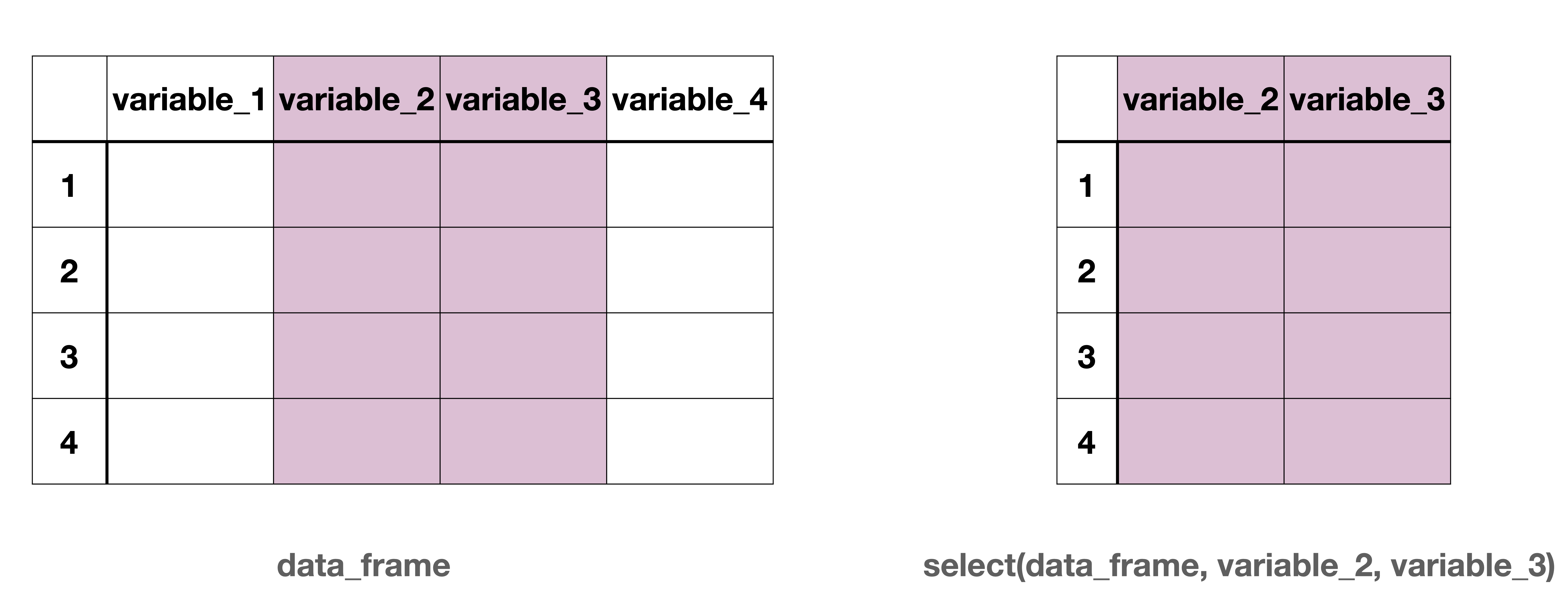
The select() function allows us to choose which columns (variables) to keep in our dataset as shown in Figure 5.1. This is particularly useful when working with large datasets that contain many variables, but you only need a few for your specific analysis. After select() is used, the resulting data frame would have the chosen columns and keep all the rows.
Figure 5.1: Column wise subsetting of a data frame
The select() function takes a data frame as its argument, followed by the names of variables we want to keep.
Notice that in the code we specify two variables to select, country and pl_consumption, and the following output only has the two specified variables and all of the 5490 rows.
We use c() function to combine multiple variable names when we want to remove more than one column. The exclamation mark (!) tells R to exclude these variables from our selection.
Notice in the output we still have all of the 5490 rows but having dropped 2 variables we now only have 12 variables. Selecting variables to drop can be more efficient than listing all the variables you want to keep, especially when you want to keep most of the variables. Instead of typing out the names of 12 variables we want to keep, we can simply specify the 2 variables we want to remove.
The select() function becomes even more powerful when combined with helper functions that can identify columns based on patterns in their names. One particularly useful helper function is starts_with():
In addition to selecting the variables, country, currency_unit, year, and population, the starts_with() function selects all variables whose names begin with “pl” (recall that “pl” stands for “price level”) including pl_consumption, pl_capital_formation, pl_gov, pl_exports, and pl_imports.
This is incredibly useful because it allows us to select multiple related variables without having to type out each variable name individually. Other useful helper functions that work with select() include ends_with() and contains().
5.4.2 Subsetting Data Frames by Rows
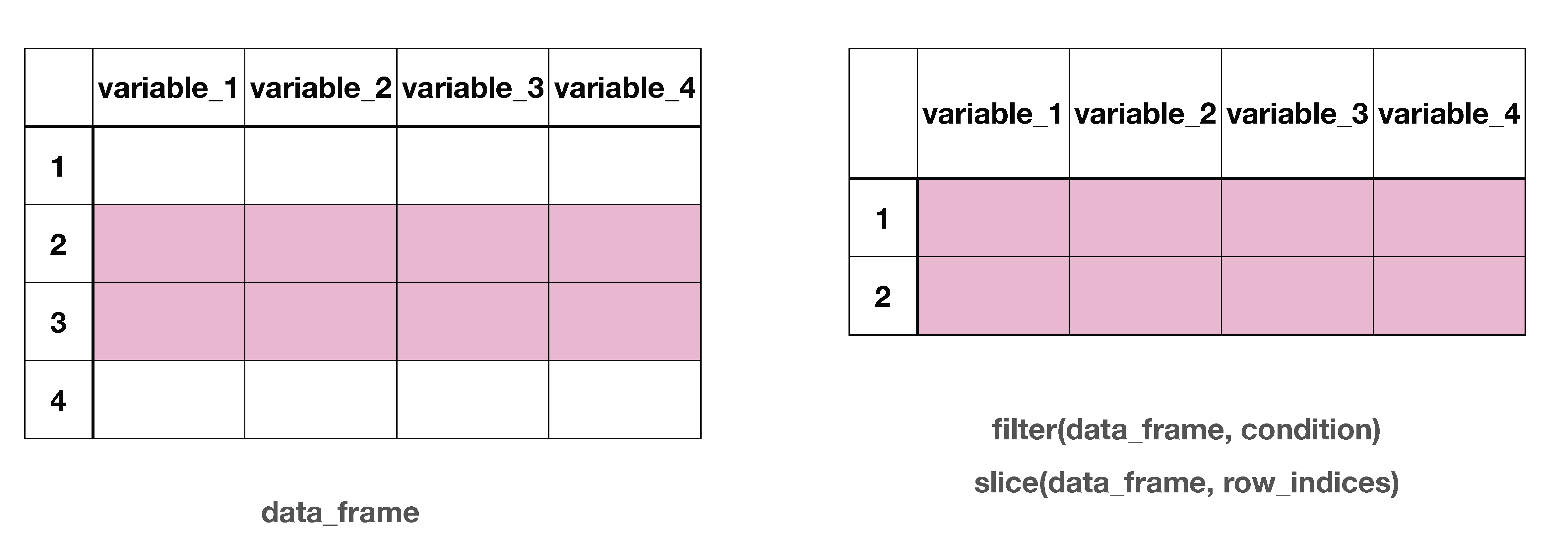
Often we want to work with only certain rows of our dataset as shown in Figure 5.2. R provides several functions to subset rows based on different criteria.
Figure 5.2: Row wise subsetting of a data frame
The filter() function allows us to subset rows based on conditions, while keeping all the columns. For instance, you might want to communicate your condition “Show me only rows if the country is United States” or “Show me only rows that have pl_exports greater than 1”. We use relational operators to create these conditions. Table 5.2 lists the relational operators in R.
Table 5.2: Relational Operators in R
Operator
Description
<
Less than
>
Greater than
<=
Less than or equal to
>=
Greater than or equal to
==
Equal to
!=
Not equal to
We can, for instance, focus our analysis on economic measures of year 2019. In this case, we only want to keep the rows for which the year is 2019.
The first argument of the filter function is penn_world which is piped into it. Then we specify the condition to filter the rows which have the year equal to 2019. Notice how we use == (two equal signs) to test for equality, not = (one equal sign). The == is used for comparison, a condition to check. In a way we are saying “filter the rows IF/WHEN the year equals to 2019”. This is NOT saying “set the year to 2019”. So this is not an equality but a test of equality.
# A tibble: 183 × 14
   country_code country currency_unit  year real_gdp_expenditure real_gdp_output
   <chr>        <chr>   <chr>         <dbl>                <dbl>           <dbl>
 1 ABW          Aruba   Aruban Guild…  2019                3921.           3467.
 2 AGO          Angola  Kwanza         2019              228151.         227856.
 3 AIA          Anguil… East Caribbe…  2019                 377.            226.
 4 ALB          Albania Lek            2019               35890.          36103.
 5 ARE          United… UAE Dirham     2019              681526.         645956.
 6 ARG          Argent… Argentine Pe…  2019              991646.         977421.
 7 ARM          Armenia Armenian Dram  2019               41049.          43583.
 8 ATG          Antigu… East Caribbe…  2019                1986.           1604.
 9 AUS          Austra… Australian D…  2019             1280843.        1364678.
10 AUT          Austria Euro           2019              498022.         477706.
# ℹ 173 more rows
# ℹ 8 more variables: population <dbl>, employment <dbl>, average_hours <dbl>,
#   pl_consumption <dbl>, pl_capital_formation <dbl>, pl_gov <dbl>,
#   pl_exports <dbl>, pl_imports <dbl>
In the output, notice that all the values in the year column are 2019, at least for the 10 rows that we can see.
We can also combine multiple conditions using logical operators. The logical operators are shown in Table 5.3.
Table 5.3: Logical Operators in R
Operator
Description
&
and
|
or
For instance you may want to run an analysis of countries that have the currency_unit as Euro (the economic region that has adopted Euro as currency is called the eurozone) and you only care about the year 2019. For each row of data that we will get to work with, both the conditions have to be true.
penn_world |>1filter(currency_unit =="Euro"& year ==2019)
1
The currency_unit has to be Euro AND year has to be 2019. Notice that we wrote Euro in quotes but not 2019 since currency_unit is a character variable and year is numeric.
# A tibble: 20 × 14
   country_code country currency_unit  year real_gdp_expenditure real_gdp_output
   <chr>        <chr>   <chr>         <dbl>                <dbl>           <dbl>
 1 AUT          Austria Euro           2019              498022.         477706.
 2 BEL          Belgium Euro           2019              589449.         517420.
 3 CYP          Cyprus  Euro           2019               33666.          28054.
 4 DEU          Germany Euro           2019             4308862.        4275312
 5 ESP          Spain   Euro           2019             1932679.        1886595.
 6 EST          Estonia Euro           2019               49209.          44876.
 7 FIN          Finland Euro           2019              261017.         248552.
 8 FRA          France  Euro           2019             3018885.        2946958.
 9 GRC          Greece  Euro           2019              302222.         284894.
10 IRL          Ireland Euro           2019              499741.         501054.
11 ITA          Italy   Euro           2019             2508404.        2466328.
12 LTU          Lithua… Euro           2019              103480.          89642.
13 LUX          Luxemb… Euro           2019               69541.          55711.
14 LVA          Latvia  Euro           2019               59916.          56079.
15 MLT          Malta   Euro           2019               22353.          17135.
16 MNE          Monten… Euro           2019               12908.          13721.
17 NLD          Nether… Euro           2019              958315.         950078.
18 PRT          Portug… Euro           2019              350395.         325160.
19 SVK          Slovak… Euro           2019              176538.         149921.
20 SVN          Sloven… Euro           2019               82556.          70869.
# ℹ 8 more variables: population <dbl>, employment <dbl>, average_hours <dbl>,
#   pl_consumption <dbl>, pl_capital_formation <dbl>, pl_gov <dbl>,
#   pl_exports <dbl>, pl_imports <dbl>
In the output, we see rows that have currency_unit Euro and the year 2019.
You might also be interested in analyzing data for countries in North America including Canada, United States, and Mexico. We just used the phrase “and” in the previous sentence but this should not trick you. Let’s dig this deeper into this. If a row has country set to be either Canada, United States or Mexico then we want to keep this row. You might be tempted to say “Show me rows that have country as Canada or United States or Mexico. Unfortunately R is not that smart (yet). We instead have to say”Show me rows that have country as Canada or country as United States or country as Mexico”
penn_world |>filter( country =="Canada"| country =="United States"| country =="Mexico" )
# A tibble: 90 × 14
   country_code country currency_unit  year real_gdp_expenditure real_gdp_output
   <chr>        <chr>   <chr>         <dbl>                <dbl>           <dbl>
 1 CAN          Canada  Canadian Dol…  1990              915725.         941469.
 2 CAN          Canada  Canadian Dol…  1991              893206.         917014
 3 CAN          Canada  Canadian Dol…  1992              901134.         925954.
 4 CAN          Canada  Canadian Dol…  1993              928149.         947826.
 5 CAN          Canada  Canadian Dol…  1994              979113.         993124.
 6 CAN          Canada  Canadian Dol…  1995             1023228.        1042290.
 7 CAN          Canada  Canadian Dol…  1996             1053691.        1068539.
 8 CAN          Canada  Canadian Dol…  1997             1106805.        1111286.
 9 CAN          Canada  Canadian Dol…  1998             1136820.        1127569.
10 CAN          Canada  Canadian Dol…  1999             1208894.        1208232
# ℹ 80 more rows
# ℹ 8 more variables: population <dbl>, employment <dbl>, average_hours <dbl>,
#   pl_consumption <dbl>, pl_capital_formation <dbl>, pl_gov <dbl>,
#   pl_exports <dbl>, pl_imports <dbl>
We can also do row-wise subsetting using the slice() function. The slice() function allows us to examine rows by their position in the dataset:
This gives us data for Aruba from 1992 to 1995. The slice() returns rows based on their position in the dataset (like “rows 3 through 6”) whereas the filter() returns rows based on the values in the data (like “year equals 2019”).
You might have noticed that in Section 5.4 we have made numerous subseting of columns and rows, but we have not stored any of these versions of the data that we looked at. In Section 5.5, we will only utilize a subset of columns so let’s just save this version of the data.
We will utilize the mutate() function to make changes to variables or create new ones. The function takes the dataset as the first argument, then specifications on how we want to create the new variable in subsequent arguments. Or we can choose to pipe the dataset into the function.
5.5.1 Changing Variable Type
There will be times when R does not assign the correct variable type or when you want to change it based on the analysis you want to do on it. We can use the mutate() function to change the type of a variable. For instance, the year variable is stored as double but we can instead store it as integer. To do that, we begin by writing the new variable name into the mutate() function then specify the type we want to change it to.
In this case, our new variable will also be named year (i.e., we will overwrite the old year variable). Then we utilize the as.integer() function on the right hand side of the equal sign. This basically asks R to set the new year variable to be the integer version of the old year variable.
Within mutate() we can also utilize as.factor(), as.numeric(), as.double(), and as.character() to change the variables to their appropriate type.
5.5.2 Creating New Variables Using Operations Between Existing Variables
There will be other scenarios where we want to create new variables using the ones already in our dataset. For instance, we may want to create a trade balance variable (trade_balance) by subtracting pl_imports from pl_exports.
We first define the new variable before the equal sign within the mutate() function. This will be the case each time we use the mutate() function throughout the chapter. Recall that this was also the case for the rename() function. The new variable name goes first. The newbies get priority.
You can see from the first row of the output that in Aruba in 1990, the trade_balance is calculated with the formula \(0.367 - 0.482 = -0.115\), meaning that they imported more than they exported. This formula is repeated for all the cells in the trade_balance column.
We can also utilize the mutate() function to change units of a variable. For instance, the documentation of penn_world in Table 5.1 has shown that population is reported in millions. If we easily wanted to make meaning of the population we can multiply it by 1,000,000.
penn_world |>1mutate(population = population *1000000)
1
In this case on the left side of the equal sign we have population. You can still think of this as a “new variable”, which overrides the older population variable by multiplying it by 1,000,000.
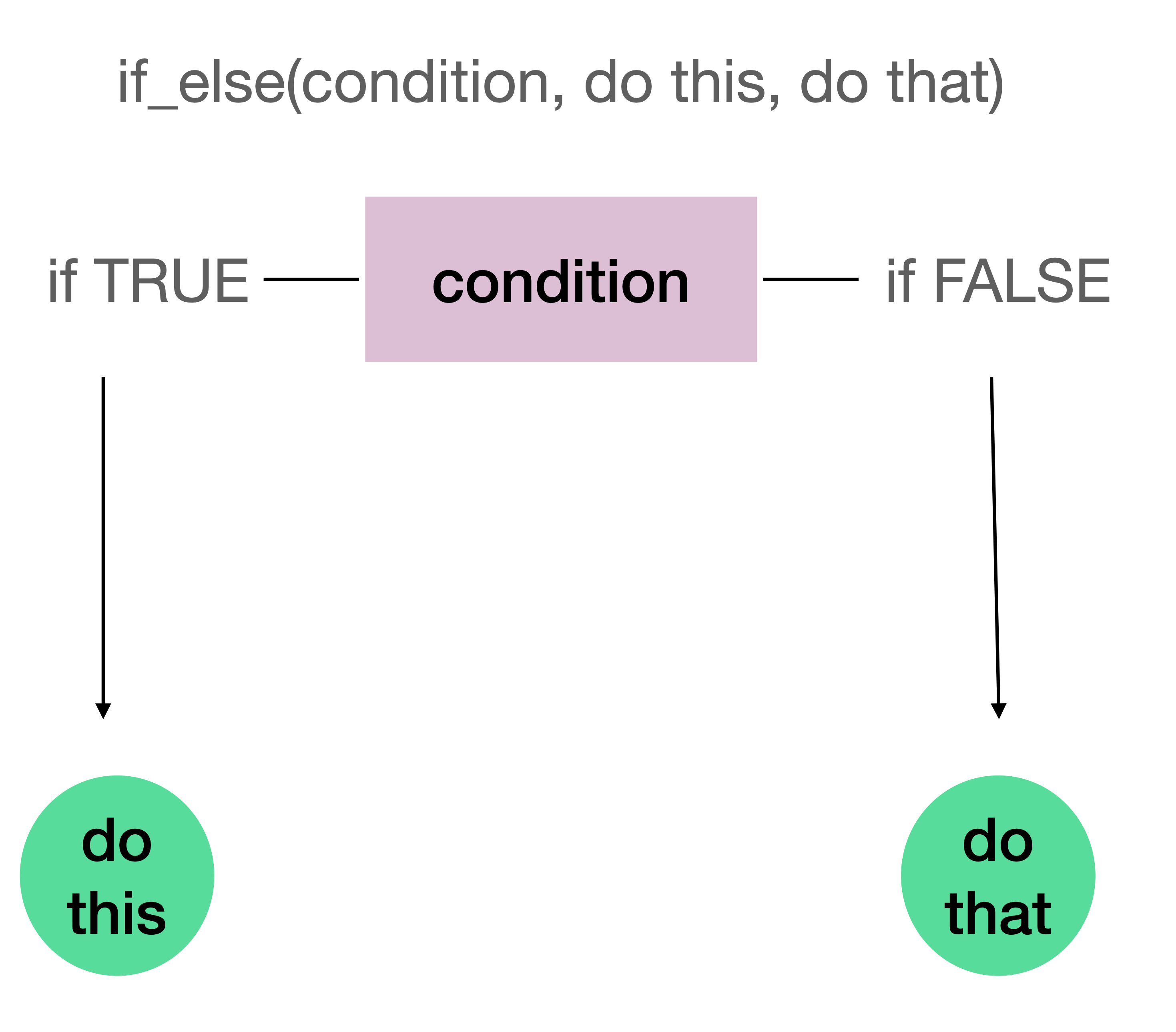
Another common use of the mutate() function is to create new variables based on a condition. When we have two outcomes of a condition, either or, then we can utilize the if_else() function to define our conditions. For instance, we might want to create a new variable called eurozone. If the currency_unit is “Euro” for any row then the eurozone will be set to “In Euro Zone”, else (i.e., if the currency_unit is not “Euro”) eurozone will be set to “Not In Euro Zone”.
penn_world |>mutate(eurozone =if_else( currency_unit =="Euro","In Euro Zone","Not In Euro Zone" ) )
# A tibble: 5,490 × 7
   country population  year currency_unit  pl_exports pl_imports eurozone
   <chr>        <dbl> <dbl> <chr>               <dbl>      <dbl> <chr>
 1 Aruba       0.0621  1990 Aruban Guilder      0.367      0.482 Not In Euro Zo…
 2 Aruba       0.0646  1991 Aruban Guilder      0.542      0.536 Not In Euro Zo…
 3 Aruba       0.0682  1992 Aruban Guilder      0.320      0.483 Not In Euro Zo…
 4 Aruba       0.0725  1993 Aruban Guilder      0.355      0.455 Not In Euro Zo…
 5 Aruba       0.0767  1994 Aruban Guilder      0.377      0.508 Not In Euro Zo…
 6 Aruba       0.0803  1995 Aruban Guilder      0.405      0.547 Not In Euro Zo…
 7 Aruba       0.0832  1996 Aruban Guilder      0.419      0.507 Not In Euro Zo…
 8 Aruba       0.0855  1997 Aruban Guilder      0.417      0.481 Not In Euro Zo…
 9 Aruba       0.0873  1998 Aruban Guilder      0.377      0.472 Not In Euro Zo…
10 Aruba       0.0890  1999 Aruban Guilder      0.355      0.486 Not In Euro Zo…
# ℹ 5,480 more rows
The syntax of the if_else() follows the pattern: if_else(condition, action_if_true, action_if_false) which is also depicted in Figure 5.3.
Figure 5.3: If else statement
In this example, the if_else() function works as follows:
Condition: currency_unit == "Euro" This checks whether each row’s currency unit equals “Euro”.
Action if TRUE: “In Euro Zone”. If the condition is true (i.e., if the currency is Euro), assign this text value to the eurozone variable.
Action if FALSE: “Not In Euro Zone” - If the condition is false (i.e., if the currency is not Euro), assign this text value to the eurozone variable.
Perhaps it might make more sense to create a eurozone variable that is a logical instead of character. Notice that logical variables have values as TRUE and FALSE without quotation marks. At the end of the code, we use the select() function to be able to show the eurozone variable on this page.
With the new eurozone variable added. The penn_world now has 7 columns.
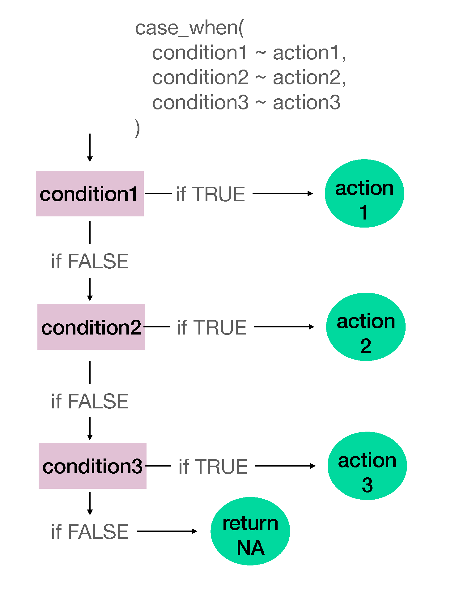
Sometimes we need to create variables based on multiple conditions rather than just two. The case_when() function is perfect for these situations where we have more than two possible conditions and actions. Let’s create a decade variable that categorizes each year into its respective decade.
penn_world |>mutate(decade =case_when( year >=1990& year <2000~"1990s", year >=2000& year <2010~"2000s", year >=2010& year <2020~"2010s" ) )
The ~ symbol (aka tilde) separates the condition (on the left) from the value to assign (on the right). This is similar to saying “if this condition is met, then assign this value.” For instance, looking at the first condition, this code can be thought as “if the year is greater than or equal to 1990 and less than 2000, then assign the value of 1990s to the variable decade. In Figure 5.4, we summarize the sequence of actions that R checks for when using case_when() function.
Figure 5.4: Utilizing case_when() with multiple conditions
You are given the following data
x
y
-1
10
2
20
5
30
and the following code:
data_frame |>mutate(z =case_when( x >3~"Greater than 3", x >1~"Greater than 1" ) )
What do you think the z variable would look like? We recommend that you utilize the chart in Figure 5.4.
This code will not run because case_when() requires more than two conditions to test.
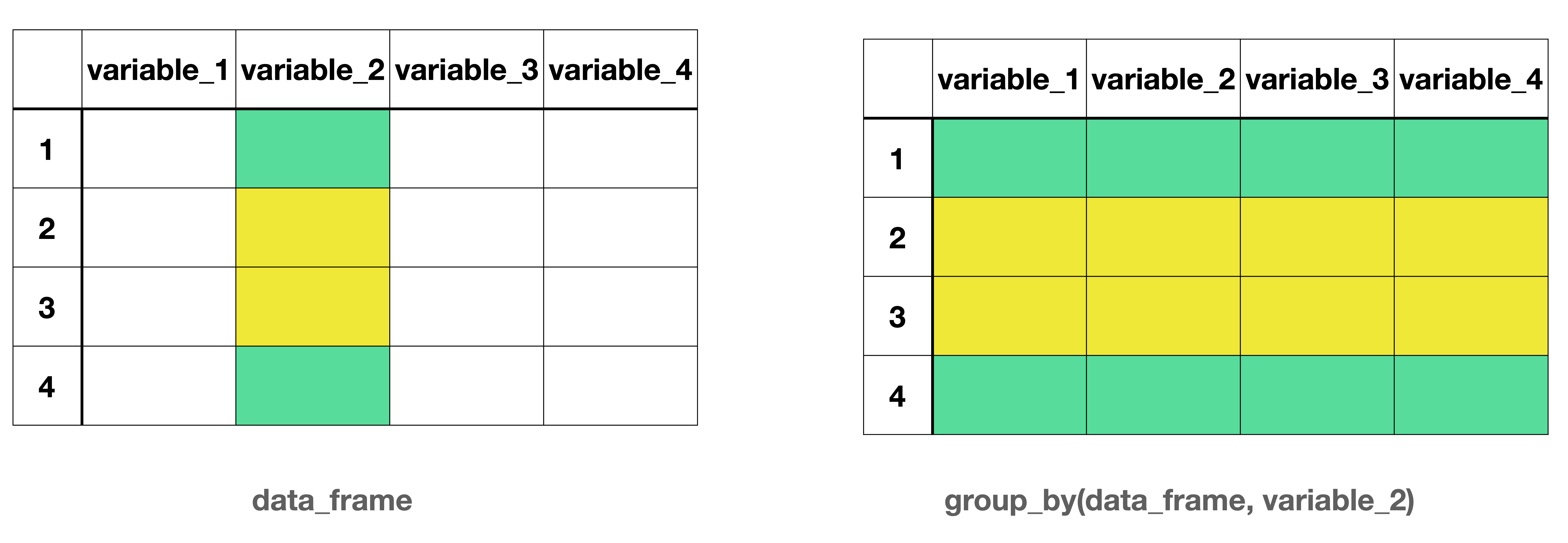
Often we want to calculate statistics for different groups in our data. The group_by() function allows us to specify how we want to group our data, and then we can perform operations on each group separately. Consider Figure 5.5 and howvariable_2 has two groups. Once the data is grouped by this variable, any analysis moving forward will be done separately for each group across any variable.
Figure 5.5: Grouping a data frame by a specific variable
Let’s start by grouping our 2019 data by whether countries are in the eurozone or not:
In this instance the categorical variable eurozone is the grouping variable.
# A tibble: 183 × 7
# Groups:   eurozone [2]
   country         population  year currency_unit pl_exports pl_imports eurozone
   <chr>                <dbl> <dbl> <chr>              <dbl>      <dbl> <lgl>
 1 Aruba               0.106   2019 Aruban Guild…      0.707      0.623 FALSE
 2 Angola             31.8     2019 Kwanza             0.476      0.612 FALSE
 3 Anguilla            0.0149  2019 East Caribbe…      0.769      0.603 FALSE
 4 Albania             2.88    2019 Lek                0.630      0.525 FALSE
 5 United Arab Em…     9.77    2019 UAE Dirham         0.689      0.647 FALSE
 6 Argentina          44.8     2019 Argentine Pe…      0.648      0.631 FALSE
 7 Armenia             2.96    2019 Armenian Dram      0.666      0.587 FALSE
 8 Antigua and Ba…     0.0971  2019 East Caribbe…      0.767      0.571 FALSE
 9 Australia          25.2     2019 Australian D…      0.608      0.694 FALSE
10 Austria             8.96    2019 Euro               0.677      0.640 TRUE
# ℹ 173 more rows
Our data looks like nothing has changed other than filtering for year 2019. Notice that there is an easy-to-miss part in the second line of the output that shows Groups: eurozone [2], indicating that our data is now grouped by the eurozone variable and there are 2 groups (TRUE and FALSE). However, just grouping the data doesn’t calculate any statistics yet - it simply organizes the data for subsequent operations. To actually calculate summary statistics for each group, we need to combine group_by() with summarize():
Since the summarize() function has been executed after the data frame has been split into groups, the summary statistic is reported for each group separately.
We have used several functions in this chapter including, clean_names(), rename(), select(), filter()mutate(), group_by(), and summarize(). All these functions take a data frame as their first argument. Even though as you are reading you may not clearly see the data frame, for instance we only wrote group_by(eurozone), but there is a data frame getting piped into the group_by() function, and so the eurozone variable is the second argument.
Feenstra, Robert C, Robert Inklaar, and Marcel P Timmer. 2015. “The Next Generation of the Penn World Table.”American Economic Review 105 (10): 3150–82.
The correct answer is d. At first glance option b might seem correct as that’s exactly what is written within the rename function but recall that the first argument is piped into the rename() function from the previous line of code. At the end of that line, there is penn_world with cleaned names.↩︎
1.) 3 would be saved into x, not printed, 2.) 1, 3, 7, 12 would be printed.↩︎
The correct answer is c. For the first row where x = - 1, case_when() checks if this number is greater than 3. It is not. Then it moves onto the next condition. It checks if -1 is greater than 1, it is not. It does not have any more conditions defined then for the first row it sets z to be NA. For the second row where x = 2, since x is not greater than 3, it moves on to the second condition. Since x > 1 for this row then it sets z as “Greater than 1”. For the last row, since x = 5, and the first condition of x > 3 is met, it sets z as “Greater than 3” and stops there.↩︎