6  Dealing with Specific Types of Variables: Strings, Dates, and Factors

In Chapter 5, you have learned multiple functions that helped you clean and tidy variables. In this chapter, we will continue our journey in cleaning variables and getting them into a shape or format that we would like to use. We will specifically work with three types of variables: strings, dates, and factors.

A string is a sequence of characters (letters, numbers, symbols, or spaces) treated as a single piece of text. As you may recall from Chapter 2, R formally identifies this data type as character (indicated as <chr>). Whether it is a single letter like "A" or a full address like "6067 Wilshire Blvd, Los Angeles, CA 90036", R treats them as a sequence of individual characters wrapped in quotes. In this book, we use the term string to describe the data and character to describe the technical vector type in R.

As you might guess, dates (and date-times) are variables that represent a specific point in time. While they may look like strings (e.g., “2026-01-01”), on the back end, R stores them numerically as the time elapsed since a reference point (January 1, 1970). They allow us to perform calendar arithmetic, such as calculating the number of days between two events or identifying which day of the week a specific date falls on.

As defined in Chapter 2, factors are used to represent categorical data with groups (i.e., levels). While they may look like strings, factors are stored as integers with associated labels (levels). They are essential when your data has a fixed and known set of possible values, such as “High”, “Medium”, and “Low” priority, and you need to control the order in which those values appear in tables or plots.

• Identify basic issues related to strings, factors, and dates
• Identify patterns in functions and arguments when dealing with strings, factors, and dates

It is important to note that it is not possible, nor necessary, to memorize every single function related to these data types. It is also not possible for us to teach you every single function either. Instead, the goal is to understand the big picture and the common issues associated with strings, dates, and factors. By recognizing the underlying patterns in how these variables behave, you will develop the intuition needed to identify which tools to use and how to find specific functions when you encounter new challenges in your own data journey.

Throughout the chapter you will see the select() function and head(3) a lot; that is solely used to show you the first three rows for a specific variable that we are working on at a given time.

6.1 Data Context

In many parts of the world, emergency services are reached through different digits, and 911 is the official emergency telephone number for the United States, Canada, and several other countries in the Caribbean and Central America. In this chapter, we will be using the sf911 data which includes all response data from the San Francisco Fire Department and Emergency Medical Services dispatched calls for service. The sf911 dataset includes every incident the department responds to based on 911 calls, providing a mix of addresses, incident categories, and time stamps. The sf911 data can be found in the {sfemergency25} package.

Before we get familiar with the new dataset that we will be working with, we will take a detour and learn more about installing R packages. When we learned how to install packages in Chapter 1 using the install.packages() function, knowingly or unknowingly, we have downloaded packages from The Comprehensive R Archive Network (CRAN). You can think of CRAN as an online network where packages are stored and when we ask R to download a package, R downloads it from CRAN by default. However, not all R packages are on CRAN. There are many other places that R packages might live such as GitHub, Bioconductor, and other local and online servers. For instance, {sfemergency25} is currently only available on GitHub. More specifically it is available at https://github.com/hellodata-science/sfemergency25. Pay attention to this URL closely. After github.com we can see that the URL continues as hellodata-science/sfemergency25, where hellodata-science is the owner of the repository and sfemergency25 is the name of the repository.

To download the {sfemergency25} package from GitHub we will use the {pak} package. You should first install the {pak} package in the Console.

install.package("pak")

Once the {pak} package is installed, using its pkg_install() function, you can install the {sfemergency25} package from GitHub repo that belongs to hellodata-science. Make sure to write this code in the Console like you normally would for any other package installations.

pak::pkg_install("hellodata-science/sfemergency25")

Then you can go ahead and load the necessary packages in your Quarto notes.

library(sfemergency25)
library(tidyverse)

── Attaching core tidyverse packages ──────────────────────── tidyverse 2.0.0 ──
✔ dplyr     1.2.1     ✔ readr     2.2.0
✔ forcats   1.0.1     ✔ stringr   1.6.0
✔ ggplot2   4.0.3     ✔ tibble    3.3.1
✔ lubridate 1.9.5     ✔ tidyr     1.3.2
✔ purrr     1.2.2     
── Conflicts ────────────────────────────────────────── tidyverse_conflicts() ──
✖ dplyr::filter() masks stats::filter()
✖ dplyr::lag()    masks stats::lag()
ℹ Use the conflicted package (<http://conflicted.r-lib.org/>) to force all conflicts to become errors

In this chapter we will focus on functions from three specific packages: {stringr}, {lubridate}, and {forcats}.

1library(stringr)
2library(lubridate)
3library(forcats)

1

We will use the {stringr} package for handling strings.

2

We will use the {lubridate} package for handling dates.

3

We will use the {forcats} package for handling factors. You can think of {forcats} as for cat egorical variable s or as an anagram of factors.

Even though we have specifically loaded {stringr}, {lubridate}, and {forcats} packages, we actually did not need to. When we loaded library(tidyverse) the output had showed us that {stringr}, {lubridate}, and {forcats} are among the loaded packages.

As mentioned before, to explore strings, dates, and factors in this chapter, we will use the sf911 data. In this dataset, each row represents a response from the San Francisco Fire Department and Emergency Medical Services. Thus, there might be multiple responses to a single call, so do not be surprised if you see the same 911 call mentioned over multiple rows.

Let’s load the dataset and glimpse at it.

data(sf911)
glimpse(sf911)

Rows: 369,089
Columns: 28
$ call_number                    <chr> "250160183", "250672403", "250120282", …
$ unit_id                        <chr> "T01", "B04", "E11", "T03", "T02", "E32…
$ incident_number                <chr> "25008211", "25035733", "25006095", "25…
$ call_type                      <chr> "Alarms", "Alarms", "Alarms", "Elevator…
$ call_date                      <chr> "01/16/2025", "03/08/2025", "01/12/2025…
$ watch_date                     <chr> "01/15/2025", "03/08/2025", "01/11/2025…
$ received_dt_tm                 <chr> "2025 Jan 16 02:41:42 AM", "2025 Mar 08…
$ entry_dt_tm                    <chr> "2025 Jan 16 02:43:02 AM", "2025 Mar 08…
$ dispatch_dt_tm                 <chr> "2025 Jan 16 02:43:55 AM", "2025 Mar 08…
$ response_dt_tm                 <chr> "2025 Jan 16 02:46:32 AM", "2025 Mar 08…
$ on_scene_dt_tm                 <chr> NA, "2025 Mar 08 05:36:04 PM", "2025 Ja…
$ transport_dt_tm                <chr> NA, NA, NA, NA, NA, NA, NA, NA, NA, NA,…
$ hospital_dt_tm                 <chr> NA, NA, NA, NA, NA, NA, NA, NA, NA, NA,…
$ call_final_disposition         <chr> "Fire", "Other", "Fire", "Fire", "Fire"…
$ available_dt_tm                <chr> "2025 Jan 16 03:01:30 AM", "2025 Mar 08…
$ address                        <chr> "02ND ST/FOLSOM ST", "GREENWICH ST/STEI…
$ city                           <int> 17, 17, 17, 17, 17, 17, 17, 17, 15, 17,…
$ zipcode_of_incident            <dbl> 94107, 94123, 94110, 94109, 94108, 9413…
$ original_priority              <int> 3, 3, 3, 3, 3, 3, 3, 3, 3, 3, 3, 3, NA,…
$ priority                       <int> 3, 3, 3, 3, 3, 3, 3, 3, 3, 3, 3, 3, 3, …
$ final_priority                 <int> 2, 2, 2, 2, 2, 2, 2, 2, 2, 2, 2, 2, 2, …
$ als_unit                       <lgl> FALSE, FALSE, TRUE, FALSE, FALSE, FALSE…
$ call_type_group                <chr> "Alarm", "Alarm", "Alarm", "Alarm", "Al…
$ number_of_alarms               <dbl> 1, 1, 1, 1, 1, 1, 1, 1, 1, 1, 1, 1, 1, …
$ unit_type                      <chr> "TRUCK", "CHIEF", "ENGINE", "TRUCK", "T…
$ unit_sequence_in_call_dispatch <dbl> 3, 2, 1, 1, 2, 3, 2, 1, 2, 1, 1, 1, 3, …
$ neighborhoods_boundaries       <chr> "Financial District/South Beach", "Mari…
$ case_location                  <chr> "POINT (-122.396705177 37.785542131)", …

Having come this long in your data science journey, without us telling you, your first steps should be to pay attention to the number of rows and columns, and read the documentation by using ?sf911 in the Console to understand what each variable represents. Given that the data frame has 28 variables, we will only be sharing details about the variables that we use within this chapter.

6.2 Strings

Data scientists deal with all sorts of problems related to strings, such as inconsistent capitalization (e.g., “SAN FRANCISCO” vs “San Francisco”), extra whitespace, or the need to extract specific information from a long sentence. To solve these issues, we use the {stringr} package. One of the most helpful features of {stringr} is that almost all of its functions start with the prefix str_.

A frequent task in data cleaning is finding a specific pattern and replacing it with something else. Let’s take a quick look at the address variable.

sf911 |> 
  select(address) |> 
  head(3)

# A tibble: 3 × 1
  address                
  <chr>                  
1 02ND ST/FOLSOM ST      
2 GREENWICH ST/STEINER ST
3 MISSION ST/POWERS AVE  

For instance, in the address variable, we might want to expand the abbreviation “ST” to “STREET” for clarity. In other words, we may want to replace “ST” with “STREET”. In this case, we would use the str_replace() function.

sf911 |> 
  mutate(
1    address_long = str_replace(
      address, 
      pattern = "ST", 
      replacement = "STREET"
    )
  ) |>
  select(address_long) |> 
  head(30)

1

Using mutate() we are creating a new variable called address_long which is defined by using the str_replace() function. This function basically takes the address variable, and wherever it encounters the pattern “ST”, it replaces it with “STREET”.

# A tibble: 30 × 1
   address_long                
   <chr>                       
 1 02ND STREET/FOLSOM ST       
 2 GREENWICH STREET/STEINER ST 
 3 MISSION STREET/POWERS AVE   
 4 OCTAVIA STREET/SUTTER ST    
 5 SACRAMENTO STREET/WAVERLY PL
 6 CARRIE STREET/WILDER ST     
 7 CLIFFORD TER/UPPER TER      
 8 18TH STREET/HARTFORD ST     
 9 MERRIE WAY/POINT LOBOS AVE  
10 LOMBARD STREET/MASON ST     
# ℹ 20 more rows

Looking at the output above, it almost seems like we have achieved the replacement task. Though you might notice a problem. The rows where “ST” appears twice have not been handled well. Take a look at the first row: 02ND STREET/FOLSOM ST. While the first appearance (i.e., first match) of “ST” has been replaced with “STREET”, that has not been the case for the second appearance, as it still appears as “ST”. The str_replace() function finds the first match of the pattern and replaces it, then stops, and moves on to the next row to continue the search. In comparison, the str_replace_all() continues through the entire string to find and replace every match. Let’s use that instead.

sf911 |> 
  mutate(
    address_long = str_replace_all(
      address, 
      pattern = "ST", 
      replacement = "STREET"
    )
  ) |>
  select(address_long) 

# A tibble: 369,089 × 1
   address_long                       
   <chr>                              
 1 02ND STREET/FOLSOM STREET          
 2 GREENWICH STREET/STREETEINER STREET
 3 MISSION STREET/POWERS AVE          
 4 OCTAVIA STREET/SUTTER STREET       
 5 SACRAMENTO STREET/WAVERLY PL       
 6 CARRIE STREET/WILDER STREET        
 7 CLIFFORD TER/UPPER TER             
 8 18TH STREET/HARTFORD STREET        
 9 MERRIE WAY/POINT LOBOS AVE         
10 LOMBARD STREET/MASON STREET        
# ℹ 369,079 more rows

If you have many replacements to make, you can use str_replace_all() with a vector containing the list of names to replace. For instance, below we are creating a vector called address_key that has full form of each abbreviation that could be seen in the first 10 rows of the address variable¹. This allows us to make multiple replacements at once, which is much more efficient than writing multiple mutate() steps.

address_key <- 
  c(
    "ST"   = "STREET", 
    "AVE"  = "AVENUE", 
    "PL"   = "PLACE", 
    "TER"  = "TERRACE"
  )

sf911 |> 
1  mutate(address_long = str_replace_all(address, pattern = address_key)) |>
  select(address_long)

1

Within mutate(), the new variable address_long is created by using the str_replace_all() function, which takes the original string to be modified/searched (e.g., address) and set of patterns with replacements to be made (e.g., address_key).

# A tibble: 369,089 × 1
   address_long                       
   <chr>                              
 1 02ND STREET/FOLSOM STREET          
 2 GREENWICH STREET/STREETEINER STREET
 3 MISSION STREET/POWERS AVENUE       
 4 OCTAVIA STREET/SUTTERRACE STREET   
 5 SACRAMENTO STREET/WAVENUERLY PLACE 
 6 CARRIE STREET/WILDER STREET        
 7 CLIFFORD TERRACE/UPPER TERRACE     
 8 18TH STREET/HARTFORD STREET        
 9 MERRIE WAY/POINT LOBOS AVENUE      
10 LOMBARD STREET/MASON STREET        
# ℹ 369,079 more rows

Looking at the first 10 rows we can see that all the abbreviations have now been expanded.

Working with strings can either give you a headache or joy, or both at the same time. The problems with strings can sometimes seem endless but the more you work with string data, the more joy you will get out of it, as it will feel like solving a puzzle. Take a look at the second row above: we’ve created another issue. By using str_replace_all(), we have changed STEINER ST into STREETEINER STREET.

To address this, we can utilize regular expressions (regex). You can think of regex as a specialized language used to perform highly specific text searches. While regex can become incredibly complex, often reaching far beyond the scope of introductory data science and thus our book, solving this specific “STREETEINER” problem offers a perfect look into its utility.

Instead of a blunt search for the characters “ST,” regex allows us to instruct R more precisely. We want R to find ‘ST’, but only when it functions as a standalone word.

address_key <- c(
1  "\\bST\\b"  = "STREET",
  "\\bAVE\\b" = "AVENUE",
  "\\bPL\\b"  = "PLACE",
  "\\bTER\\b" = "TERRACE"
)

sf911 |> 
  mutate(address_long = str_replace_all(address, pattern = address_key)) |> 
  select(address_long)

1

The use of \\b at the beginning and end of “ST” creates a word boundary. In this instance, in STEINER, the “ST” is followed by “E”. Since “E” is a word character, there is no boundary, such as a space, after the letter “T”. Hence, the regex engine will skip it.

# A tibble: 369,089 × 1
   address_long                   
   <chr>                          
 1 02ND STREET/FOLSOM STREET      
 2 GREENWICH STREET/STEINER STREET
 3 MISSION STREET/POWERS AVENUE   
 4 OCTAVIA STREET/SUTTER STREET   
 5 SACRAMENTO STREET/WAVERLY PLACE
 6 CARRIE STREET/WILDER STREET    
 7 CLIFFORD TERRACE/UPPER TERRACE 
 8 18TH STREET/HARTFORD STREET    
 9 MERRIE WAY/POINT LOBOS AVENUE  
10 LOMBARD STREET/MASON STREET    
# ℹ 369,079 more rows

Another instance is when character data is presented in all UPPERCASE or all lowercase. We can use the functions str_to_upper(), str_to_lower(), or str_to_title() to fix this. In the sf911 data, the address column is entirely capitalized, which can be difficult to read in a final report. We can change it to title case, where the first letter of each word is capitalized.

sf911 |> 
1  mutate(address = str_to_title(address)) |>
  select(address) |> 
  head()

1

Within mutate(), a new version of address is created by taking the old address variable and applying title case to it using the str_to_title() function.

# A tibble: 6 × 1
  address                 
  <chr>                   
1 02nd St/Folsom St       
2 Greenwich St/Steiner St 
3 Mission St/Powers Ave   
4 Octavia St/Sutter St    
5 Sacramento St/Waverly Pl
6 Carrie St/Wilder St     

Sometimes we need to “paste” columns together to create a more descriptive variable. While R has a built-in paste() function, {stringr} provides str_c() for simple combination of vectors and str_glue() for more complex templates. The str_glue() function allows you to wrap column names in curly braces {} to “glue” them into a sentence.

sf911 |> 
1  mutate(
2    description = str_glue(
3      "Incident {call_number} occurred in {neighborhoods_boundaries}"
    )
  ) |> 
  select(description) |> 
  head(3)

1

Using the mutate() function we are creating a new variable called description.

2

The description variable is created by using the str_glue() function which glues together a full sentence.

3

Within this sentence variables of the sf911 data frame call_number and neighborhoods_boundaries are used within curly brackets {}.

# A tibble: 3 × 1
  description                                                  
  <glue>                                                       
1 Incident 250160183 occurred in Financial District/South Beach
2 Incident 250672403 occurred in Marina                        
3 Incident 250120282 occurred in Bernal Heights                

The last common example we will show is when we need to know if a certain word exists within a string. We use the function str_detect() for this, which returns TRUE if the pattern is found and FALSE otherwise. This is perfect for creating flagging variables.

sf911 |>
1  mutate(is_fire_related = str_detect(call_type, pattern = "Fire|Smoke")) |>
  select(call_type, is_fire_related) |> 
2  slice(1:10)

1

We are creating a new variable called is_fire_related using the mutate() function. This variable is created by using the str_detect() function by detecting existence of “Fire” or “Smoke” within call_type. The is_fire_related variable would be TRUE if call_type contains “Fire” or “Smoke”, and FALSE otherwise.

2

We are displaying rows 1 through 10 so that you can see a variety of TRUE and FALSE output for the new is_fire_related variable.

# A tibble: 10 × 2
   call_type                     is_fire_related
   <chr>                         <lgl>          
 1 Alarms                        FALSE          
 2 Alarms                        FALSE          
 3 Alarms                        FALSE          
 4 Elevator / Escalator Rescue   FALSE          
 5 Alarms                        FALSE          
 6 Traffic Collision             FALSE          
 7 Alarms                        FALSE          
 8 Vehicle Fire                  TRUE           
 9 Smoke Investigation (Outside) TRUE           
10 HazMat                        FALSE          

This is an exercise for learning to learn. We have not taught you the function str_sub(). By looking at the example below, can you figure out what the function does, and what its arguments represent? You can also learn about the function by reading the documentation.

str_sub("Hello Data Science", start = 1, end = 7)

[1] "Hello D"

Check footnote for answer²

6.3 Dates

Working with dates is notoriously difficult because humans use inconsistent formats. Depending on where you are in the world, the same date might be written as “December 20th, 1986,” “12/20/1986,” “20/12/1986,” or “20-Dec-1986.” In addition, data scientists must often account for varying time zones and the headache of Daylight Savings Time, which can shift the recorded time of an event without any actual time passing.

While there are many ways to write a date for humans, there is only one universally accepted format for data as standardized by the International Organization for Standardization (ISO). It follows the order of YYYY-MM-DD (e.g., 1986-12-20). Writing dates this way ensures they are sorted correctly by computers and avoids any international confusion between months and days.

When working with time data, you will encounter UTC quite often. UTC stands for Coordinated Universal Time. Think of it as the world’s main clock. A reader of Hello Data Science in Mersin, Türkiye would see a different time on their clock than a reader in Guadalajara, Mexico. But if both readers turned to the main clock of the world, they would see the exact same time.

UTC is not technically a time zone, but rather the high-precision time standard that all time zones use to stay synchronized. Every time zone on Earth is defined by its offset from UTC. For instance, Los Angeles is UTC-8 (8 hours behind UTC) between first Sunday of November and second Sunday of March which is specified as Pacific Standard Time (PST) and UTC-7 during rest of the year which is specified as Pacific Daylight Time (PDT). In data science, we treat UTC as the main point of reference for time. Because UTC never observes Daylight Savings Time, it is the safest format for storing data and performing arithmetic operations.

Where do you currently live? Use online search to find your timezone in comparison to UTC. Are daylight savings observed in your location?

Check footnote for answer³

In R, if data is stored as a date then we see it as a date. On the back end, what we don’t see is how R stores date and time variables. Computers don’t inherently know what a year or a month is. To handle dates, they need a starting point to begin counting. By international agreement, that starting point is Midnight on January 1, 1970 (UTC).

To ensure that a computer in Tehran and a computer in London interpret that “count” in the exact same way, we use a standard called POSIX (Portable Operating System Interface). In R, you will most often see date time variable format POSIXct. The “ct” stands for calendar time. This format stores a date-time as a single, massive number: the total number of seconds that have elapsed since midnight on January 1, 1970.

The first step in any date analysis is converting a string into a formal date object. In the sf911 data, we have several columns ending in _dt_tm indicating date and time, such as the variable received_dt_tm, which indicates the date and time a call is received at the 911 Dispatch Center.

sf911 |> 
  select(received_dt_tm) |> 
  head(3)

# A tibble: 3 × 1
  received_dt_tm         
  <chr>                  
1 2025 Jan 16 02:41:42 AM
2 2025 Mar 08 05:28:54 PM
3 2025 Jan 12 02:19:44 AM

The values look like: 2025 Jan 16 02:41:42 AM. To convert this character variable into an appropriate date format, you don’t need to memorize a complex code; you just need to look at the order of the components: Year, Month, Day, Hour, Minute, Second. In the {lubridate} package, the function name matches that order: ymd_hms().

sf911 <-
  sf911 |>
1  mutate(received_dt_tm = ymd_hms(received_dt_tm))

2str(sf911$received_dt_tm)

1

The new version of the received_dt_tm variable is based on the old received_dt_tm changed to a year, month, day, hour, minute, seconds format using the ymd_hms() function. If your data was in a different order, like “Day-Month-Year,” you would simply use dmy(). Hence, we first identify the order, and then use the initial letters of the order to identify the {lubridate} function.

2

Checking the structure of the newly stored received_dt_tm variable returns POSIXct as seen below.

 POSIXct[1:369089], format: "2025-01-16 02:41:42" "2025-03-08 17:28:54" "2025-01-12 02:19:44" ...

On the front end we see a date and time as 2025-01-16 02:41:42. The way R stores this on the back end is in number of seconds since midnight on January 1, 1970. Even though R stores the received_dt_tm variable as POSIXct, in tidyverse when tibbles are printed, this will display as dttm as seen in the output below.

sf911 |> 
  select(received_dt_tm) |> 
  head(3)

# A tibble: 3 × 1
  received_dt_tm     
  <dttm>             
1 2025-01-16 02:41:42
2 2025-03-08 17:28:54
3 2025-01-12 02:19:44

The dttm signifies date and time. This is only a visual label. In R, you might encounter other types of date and time related types and labels including date (date without time or timezone), hms (time without date), POSIXlt (POSIX list time), and difftime (time differences).

We can use the function with_tz() to shift a date-time to the correct local time, otherwise R will treat it as UTC. To see a full list of time zones in R, you can use the OlsonNames() function which has 598 different names of timezones.

sf911 <-
  sf911 |> 
  mutate(
1    received_dt_tm = with_tz(received_dt_tm, tzone = "America/Los_Angeles")
    )

sf911 |> 
  select(received_dt_tm) |> 
  head(3)

1

We use the with_tz() function to specify for which variable we want to set the timezone and tzone argument to set the specific timezone. In the output you will not see this timezone set but it is set.

# A tibble: 3 × 1
  received_dt_tm     
  <dttm>             
1 2025-01-15 18:41:42
2 2025-03-08 09:28:54
3 2025-01-11 18:19:44

Once R understands that a variable is a date, we can easily pull out specific pieces of information. This is helpful for finding patterns, such as “What is the busiest hour of the day?” or “Which day of the week has the most fires?”

sf911 |> 
  mutate(
1    hour_val = hour(received_dt_tm),
2    month_val = month(received_dt_tm, label = TRUE),
3    day_name = wday(received_dt_tm, label = TRUE)
  ) |> 
  select(received_dt_tm, hour_val, month_val, day_name) |> 
  head(3)

1

hour() extracts the hour component [0–23] from the date-time.

2

month() extracts the month. By setting label = TRUE, we get the name (e.g., "Jan") instead of the number (e.g., 1).

3

wday() extracts the day of the week. label = TRUE provides the name (e.g., "Wed", "Sat"). Note that if you do not use the label = TRUE argument then the days of the week will be enumerated. For instance if a response was on a Sunday then R might record day of the week as 1 (e.g., in U.S.) or 7 (e.g., in Europe) depending on what calendar system your computer is using.

# A tibble: 3 × 4
  received_dt_tm      hour_val month_val day_name
  <dttm>                 <int> <ord>     <ord>   
1 2025-01-15 18:41:42       18 Jan       Wed     
2 2025-03-08 09:28:54        9 Mar       Sat     
3 2025-01-11 18:19:44       18 Jan       Sat     

In R, you cannot simply add the number 5 to a date, because R won’t know if you mean 5 seconds, 5 days, or 5 years. You must use duration functions like ddays() or dseconds() to tell R exactly what unit of time you are adding or subtracting. These functions treat time as duration.

Imagine a hypothetical scenario that 911 has a goal to arrive on the scene within 480 seconds (8 minutes) of receiving a call. We can create a goal_arrival column by adding dseconds(480) to the received_dt_tm.

sf911 |>
  mutate(
    goal_arrival_time = received_dt_tm + dseconds(480)
  ) |>
  select(received_dt_tm, goal_arrival_time) |>
  head(3)

# A tibble: 3 × 2
  received_dt_tm      goal_arrival_time  
  <dttm>              <dttm>             
1 2025-01-15 18:41:42 2025-01-15 18:49:42
2 2025-03-08 09:28:54 2025-03-08 09:36:54
3 2025-01-11 18:19:44 2025-01-11 18:27:44

We can similarly use ddays(1) to add a duration of exactly one day (86,400 seconds).

When performing math with dates, {lubridate} distinguishes between two ways of measuring time: durations and periods. This distinction is critical when your data spans a Daylight Saving Time (DST) transition.

event_start <- ymd_hms("2026-03-07 05:00:00", tz = "America/Los_Angeles")

event_start + ddays(1)

[1] "2026-03-08 06:00:00 PDT"

event_start + days(1)

[1] "2026-03-08 05:00:00 PDT"

The above example shows a hypothetical event start time as March 7th, 2026 at 5:00 in Los Angeles time zone. When you add duration of exactly 1 day using the ddays() function, you are adding a duration of 86,400 seconds. When 86,400 seconds have passed the clocks would be showing 06:00 am on March 8th, 2026 due to start of Daylight Saving Time. On the other end, the days() function just adds one day period to the calendar day without touching the time component.

One of the most common tasks in analyzing emergency data is calculating how long a process takes—for example, the response time between when a call is received and when the unit arrives on the scene. When you subtract one date-time from another, R creates a special type of object called a difftime.

sf911 <- 
  sf911 |> 
  mutate(
1    on_scene_dt_tm = ymd_hms(on_scene_dt_tm),
2    response_time = on_scene_dt_tm - received_dt_tm
  )

str(sf911$response_time)

1

The on_scene_dt_tm is changed to a POSIXct format using the ymd_hms() function

2

The response_time variable is created by finding the difference of the time a response unit was on scene (i.e., on_scene_dt_tm) and the time the call was received (received_dt_tm).

 'difftime' num [1:369089] NA 430 385 334 ...
 - attr(*, "units")= chr "secs"

Looking at the output we can notice that the unit of the difftime variable is in seconds.

Another useful function when working with dates is the today() function.

today()

[1] "2026-06-16"

This book chapter was compiled on 2026-06-16. If you were to run the today() function in your own R console or Quarto document right now, it would return the date of today. This is incredibly useful for creating “date of report” labels in a Quarto document or calculating how many days have passed since a specific incident.

If you need more precision, the now() function returns the current date-time, including the hour, minute, second, and the time zone your computer is currently using.

now()

[1] "2026-06-16 09:19:32 EDT"

While {lubridate} is an incredibly powerful tool for working with date and time, it is important to remember its primary limitation: it is built exclusively for the Gregorian calendar. The Gregorian calendar is the solar calendar used by most of the world today. Introduced in 1582, it is designed to keep the calendar year synchronized with the Earth’s revolutions around the Sun (approximately 365.24 days).

Not all cultures calculate time based on the Sun. Consider the Islamic calendar. While some countries such as Iran and Afghanistan have adopted the solar Islamic calendar (with 365.24 days), some use lunar Islamic calendar which follows the phases of the moon, and a lunar year is approximately 11 days shorter than a solar year. Because of this difference, lunar Islamic holidays like Ramadan or Eid al-Fitr do not stay fixed in a Gregorian month. Instead, they migrate backward through the Gregorian seasons over a 33-year cycle. For example, Ramadan might occur in July or in December in one’s life time in the Gregorian calendar.

If you are a data scientist analyzing consumer behavior, healthcare, or urban planning in a multicultural city, the Gregorian calendar may not tell the whole story. The Gregorian system is just one flavor in a diverse world of time-keeping. The Hebrew (Judaic) calendar is lunisolar which uses lunar months but add intercalary (leap) months to stay roughly aligned with the solar seasons. The Ethiopian calendar is solar but consists of 13 months and is approximately seven to eight years “behind” the Gregorian year.

There are many other calendars around the world. As data scientists, you need to understand culture. Data can be a reflection of human behavior, and human behavior can be governed by culture, not just the rotation of the Earth.

R does not have a single, built-in universal translator for all these systems. The {lubridate} will simply return NA if you try to feed it a date that doesn’t fit Gregorian rules (like a 30th day of February or a 13th month). Depending on the specific calendar system you would like to use you will have to search for a specific package.

6.4 Factors

In Chapter 2, you learned that factors are a special data type in R used to represent categorical variables. To manipulate these categorical variables, we use the {forcats} package. Just like with strings, one of the most helpful features of {forcats} is that almost all of its functions start with a consistent prefix: fct_. While factors might appear as text, R stores them as integers under the hood, with a specific set of labels called levels attached to each integer value.

As you might have noticed from the glimpse() output of the sf911 data, many variables that should be factors, such as neighborhoods_boundaries, call_type, priority and unit_type are currently stored as character (<chr>) vectors.

When a variable is a character, R treats every unique piece of text as an independent value. When you convert that variable to a factor, you are telling R: “This variable has a fixed and known set of possible categories.”

Let’s take a look at the unit_type variable which describes the specific kind of equipment dispatched to a scene. Its levels include categories like ENGINE (the standard fire truck with water and hoses), MEDIC (ambulances), CHIEF (command vehicles), and TRUCK (ladder trucks). Let’s convert the unit_type variable to a factor.

sf911 <-
  sf911 |>
  mutate(unit_type = as.factor(unit_type)) 
  
str(sf911$unit_type)

 Factor w/ 12 levels "AIRPORT","BLS",..: 12 3 5 12 12 5 5 5 11 5 ...

By checking the structure of unit_type, we confirm that it is now stored as a factor. We can also see that it has 12 levels. However we don’t see the label of each level, we only see a few of the labels. We also see that the first observation has the 12th level but we don’t know what the label of the 12th level is. You can see all these labels using the levels() function.

levels(sf911$unit_type)

 [1] "AIRPORT"        "BLS"            "CHIEF"          "CP"            
 [5] "ENGINE"         "INVESTIGATION"  "MEDIC"          "PRIVATE"       
 [9] "RESCUE CAPTAIN" "RESCUE SQUAD"   "SUPPORT"        "TRUCK"         

By default, R assigns levels in alphabetical order. All the 12 levels of unit_type above are in alphabetical order and we can see that the 12th level is “TRUCK”.

student_data <- data.frame(
  year = c(
    "Senior", "First-Year", "Junior", "Sophomore", "Junior", "First-Year"
  )
) |>
  mutate(year = as.factor(year))

1. What would be the order of levels of the year variable?
2. Would you be fine with the current ordering of the levels?

Check footnote for answer⁴

Let’s create a basic horizontal bar plot of the unit_type variable.

ggplot(sf911, aes(y = unit_type)) +
  geom_bar()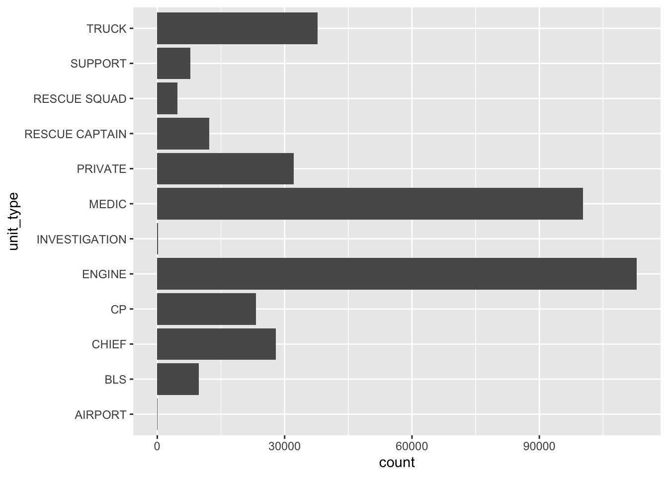

Figure 6.1: A bar plot with default alphabetical ordering

In Figure 6.1, the units are listed alphabetically from bottom to top: AIRPORT, BLS, CHIEF, and so on. While this is easy to generate using ggplot, it doesn’t help us quickly see which units are the workhorses of the department.

To make the plot more informative, we can use fct_infreq(). This function reorders the factor levels by how often they appear in the data.

sf911 <- 
  sf911 |> 
1  mutate(unit_type = fct_infreq(unit_type))

2str(sf911$unit_type)

1

The fct_infreq() function only requires a factor variable. It orders the levels in a descending order based on the number of observations within each one.

2

When we check the structure of the new version of the unit_type variable we can see that the first level is now “ENGINE”, followed by “MEDIC”.

 Factor w/ 12 levels "ENGINE","MEDIC",..: 3 5 1 3 3 1 1 1 9 1 ...

Ordering levels by frequency makes the bar plot easier to process.

ggplot(sf911, aes(y = unit_type)) +
  geom_bar()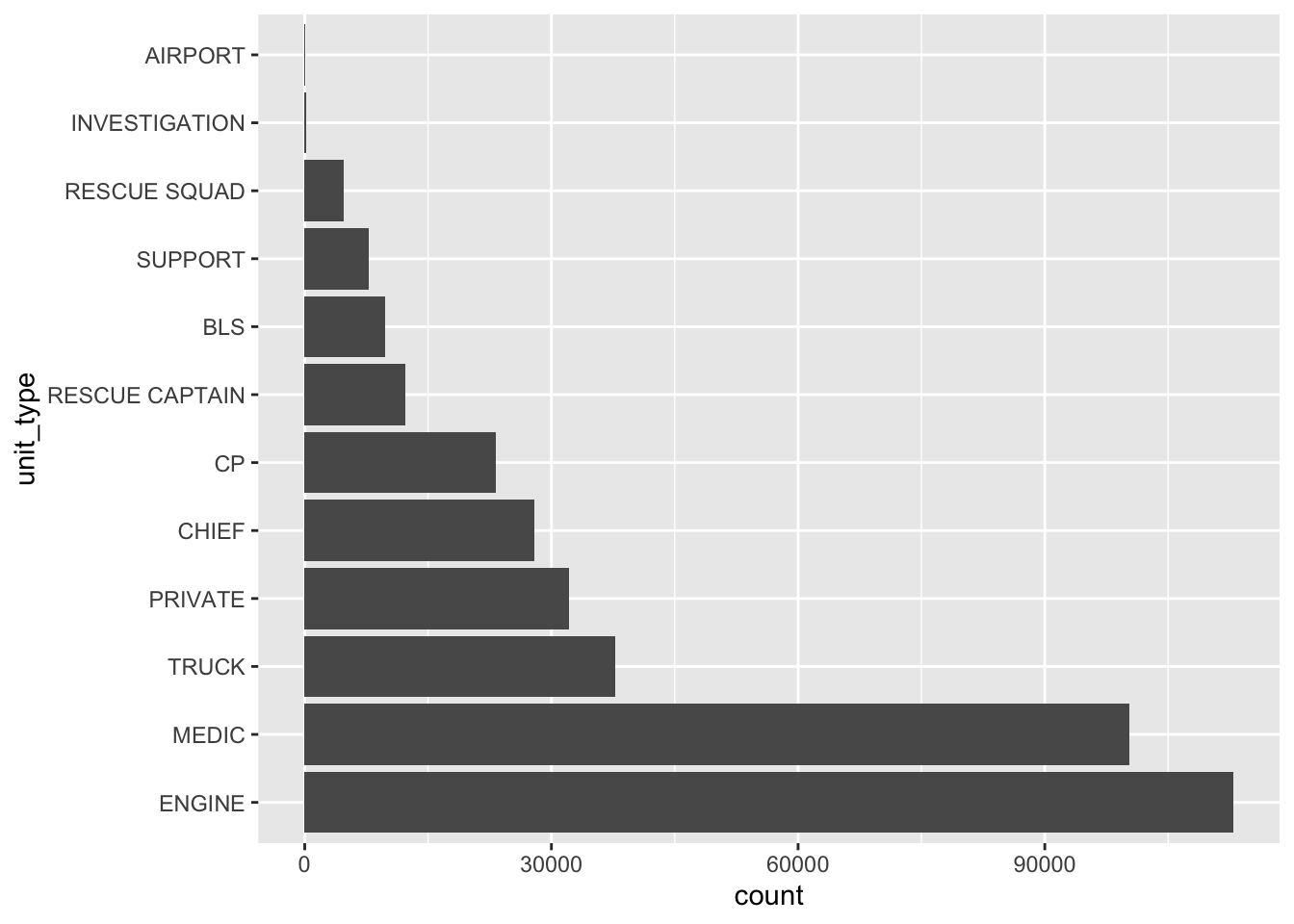

Figure 6.2: Ordered units by frequency

By default, ggplot plots the first level at the bottom. To show the levels with the highest frequencies at the top of our chart, we use fct_rev(), which helps reverse the order of factor levels.

sf911 |>
1  mutate(unit_type = fct_rev(unit_type)) |>
  ggplot(aes(y = unit_type)) +
  geom_bar()

1

The fct_rev() function only requires a factor variable whose levels will be reversed.

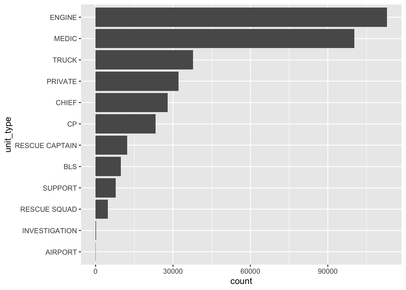
Figure 6.3: Reversing the order with fct_rev() to show busiest units at the top

Even with unit types, there are several rare categories (like “INVESTIGATION” or “AIRPORT”) that clutter the chart. The {forcats} package has a set of functions that lump uncommon factor levels into “other” category. We can use fct_lump_n() to keep the top 3 most frequent units and collapse everything else into “Other”.

sf911 |>
  mutate(unit_type = fct_lump_n(unit_type, n = 3)) |>
  ggplot(aes(y = unit_type)) +
  geom_bar()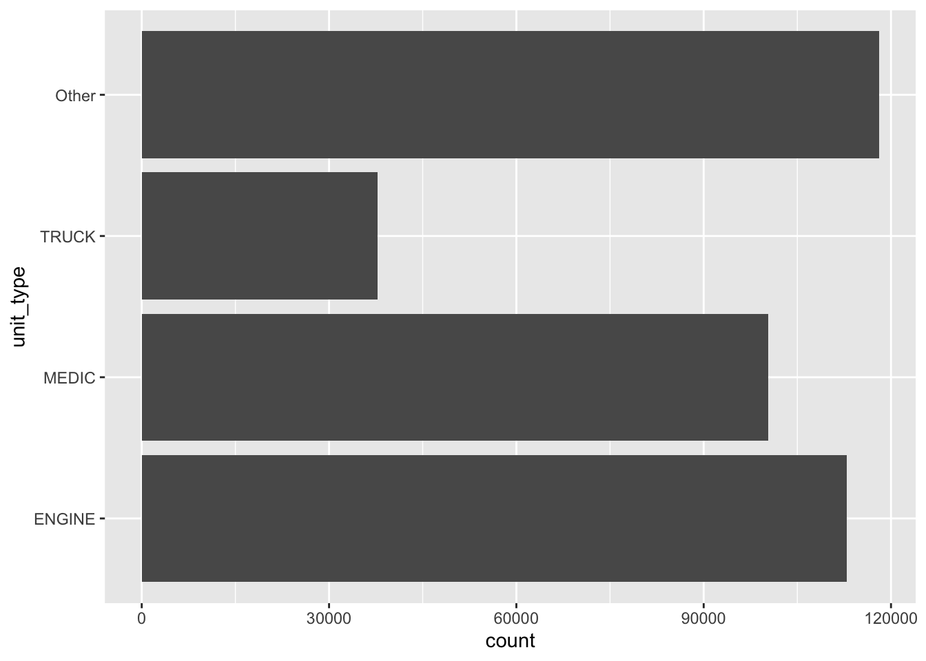

Figure 6.4: Grouping rare unit types with fct_lump_n()

The {forcats} package has additional functions that help lump uncommon factor levels into “Other” level. We encourage readers to read the documentation for fct_lump_min(), fct_lump_prop(), and fct_lump_lowfreq().

While the {forcats} functions above are great for visual cleanup, you will often need to manipulate factors for reasons that have nothing to do with plots. In professional data science, the order of levels often dictates the results of statistical models. When you run a statistical model (which you will do starting in Chapter 11), R uses the first level of a factor as the baseline or reference group. It then compares all other groups to this group. Setting a reference group isn’t just about the math; it’s also about contextual hierarchy. Since the first level is the reference group, we need to choose it deliberately rather than relying on the default first level alphabetically.

In sf911, the Engine is the standard response unit. When a Battalion Chief looks at a table of statistics, they may not be reading every row in isolation. They are mentally comparing everything to the standard Engine. If the Engine is buried in the middle of a 20-row table because of alphabetical sorting, the table is much harder to scan for insights.

By using fct_relevel(), we can ensure that the reference group we want to use is always the first thing the reader sees. This allows the reader to keep that “Engine” number in their head as they look at the other units.

sf911 |>
1  mutate(unit_type = fct_relevel(unit_type, "ENGINE")) |>
  group_by(unit_type) |>
2  summarize(total_als_unit = sum(als_unit))

1

fct_relevel() takes the level “ENGINE” and moves it to the first position (index 1). All other levels are shifted down but maintain their existing relative order.

2

After having grouped the data by unit_type we are calculating how many in total responses included a unit that includes ALS (Advance Life Support) resources. The als_unit is binary and summing it would show the number of total units with ALS.

# A tibble: 12 × 2
   unit_type      total_als_unit
   <fct>                   <int>
 1 ENGINE                  89853
 2 MEDIC                   88065
 3 TRUCK                    2336
 4 PRIVATE                     0
 5 CHIEF                       0
 6 CP                        135
 7 RESCUE CAPTAIN           9821
 8 BLS                         0
 9 SUPPORT                  5059
10 RESCUE SQUAD                0
11 INVESTIGATION               0
12 AIRPORT                     0

You can also move multiple levels to the front if you want to establish a specific priority.

sf911 |>
1  mutate(unit_type = fct_relevel(unit_type, "ENGINE", "TRUCK")) |>
  group_by(unit_type) |>
  summarize(total_als_unit = sum(als_unit))

1

This explicitly places “ENGINE” first and “TRUCK” second. This is useful when you have a primary and secondary standard that you want to highlight before showing the rest of the unit types.

# A tibble: 12 × 2
   unit_type      total_als_unit
   <fct>                   <int>
 1 ENGINE                  89853
 2 TRUCK                    2336
 3 MEDIC                   88065
 4 PRIVATE                     0
 5 CHIEF                       0
 6 CP                        135
 7 RESCUE CAPTAIN           9821
 8 BLS                         0
 9 SUPPORT                  5059
10 RESCUE SQUAD                0
11 INVESTIGATION               0
12 AIRPORT                     0

To tie our concepts of time and categorical data together, we can use the response times we calculated to rank the neighborhoods in San Francisco. This allows us to see which areas experience the longest wait times for emergency services.

In the code below, we create a new factor variable that is ordered not by the alphabet, but by the median response time in each neighborhood.

sf911 <- sf911 |>
  mutate(
1    neighborhoods_boundaries = as.factor(neighborhoods_boundaries),
2    neighborhoods = fct_reorder(neighborhoods_boundaries, response_time)
    ) 

str(sf911$neighborhoods_boundaries)
str(sf911$neighborhoods)

1

We first convert the neighborhoods_boundaries character string into a factor. By default, R assigns levels alphabetically (e.g., “Bayview Hunters Point” is Level 1 as seem in the output below).

2

We use fct_reorder() to create a new version of the neighborhoods_boundaries variable saved as neighborhoods. This function recalculates the levels so they are sorted based on the values in response_time. Neighborhoods with the smallest median response times (i.e., fastest response) are assigned the lower integers, while those with the largest are assigned the higher integers.

 Factor w/ 42 levels "Bayview Hunters Point",..: 6 17 2 13 4 7 3 3 27 24 ...
 Factor w/ 42 levels "Nob Hill","Western Addition",..: 27 20 26 14 8 34 15 15 16 23 ...

If we glimpse at the data, we would see neighborhoods_boundaries and neighborhoods look exactly the same, however, when we look at the str() output, we can see how R stores these two variables differently. The neighborhoods_boundaries variable stores levels alphabetically starting with “Bayview Hunters Point” labeled as 1, whereas neighborhoods stores levels by median response time starting with “Nob Hill” labeled as 1, since it has the lowest median response time.

---

1. We are aware that United States Postal Service has a lot more abbreviations which also appear in the rest of the address variable. For simplicity of demonstration we have kept the list brief. Readers who are interested in getting all the abbreviations correctly can use the list at https://pe.usps.com/text/pub28/28apc_002.htm

2. The str_sub() takes a string as its first argument and then subsets it, starting with the second argument position, and ending with the third argument position. The overall form can be thought as str_sub(string, start, end). Note that the space between “Hello” and “Data” counts as a position as well.

3. We have used https://www.timeanddate.com/worldclock/turkey/mersin to find the timezone in Mersin, Türkiye. Mersin is in UTC+3 timezone. As of writing this book, Mersin does not have a Daylight Savings Time, even though it had one in the past.

4. The year variable would have levels in the order of First-Year, Junior, Senior, Sophomore based on alphabetical ordering. It would be better to set the order of levels to be First-Year, Sophomore, Junior, Senior.