8 Tables, Functions, and Iterations

In Chapter 7, you learned to work with multiple data frames with different variables. In this chapter, we will continue working with multiple data frames but now all of the data frames will have the same variable names. We will focus on three fundamental data science pillars: tables, functions, and iterations.

While these three concepts might initially seem like separate, isolated tools, they represent a natural progression in a data scientist’s workflow. You will be able to extract a data source, automate its analysis, present your findings in a publication-ready table, and repeat the same process for a similar data source.

By the end of Chapter 10, you will be well-equipped to complete your first full data science project. For that project, or any future analysis you share with an audience, presenting raw data frames is rarely sufficient. A neatly designed table can be an incredibly powerful tool for summarizing complex findings and guiding a reader’s eye directly to the insight. In this chapter, we will show you how to move past default console outputs to design elegant, expressive tables.

So far throughout this book, you have been a consumer of functions, relying on tools built by other developers across the R ecosystem. The time has now come to become a creator and write your own functions. Not only will we construct a custom pipeline to process our data, but we will also learn how to execute that pipeline over and over again without duplicating code—a computational process known as iteration.

Design aesthetic, presentation-ready tables
Formulate custom functions and specify their arguments
Implement iterative structures to execute repetitive actions

Let’s go ahead and load the packages we will use for this chapter. In addition to our regular use of {tidyverse}, we will use {gt} and {gtExtras} packages which provide a powerful framework for table visualization.

library(tidyverse)
library(gt)
library(gtExtras)

The R ecosystem offers a rich and diverse landscape of packages dedicated entirely to generate tables. Beyond {gt} and {gtExtras}, you will frequently encounter packages such as {kable}, {kableExtra}, {formattable}, {DT}, and {reactable}, each optimized for different data workflows. In this chapter, we focus on {gt}.

It is important to note that this chapter is an entry point, not a comprehensive manual for table design. As you develop your own data projects, we highly recommend exploring the documentation for these packages and others to expand your toolkit. Furthermore, our output type throughout this book has primarily been HTML documents. If your workflow requires rendering Quarto to a PDF document every function in this chapter may not render properly.

8.1 Data Context

Our empirical exploration in this chapter utilizes system data from Capital Bikeshare, a bicycle-sharing system serving the Washington, D.C. metropolitan area. Bikeshare systems represent a classic smart-city utility: customers rent a bicycle from a docking station in one neighborhood and return it to a docking station elsewhere in the service area. These systems generate massive datasets containing millions of individual trips.

Capital Bikeshare makes their historical ride data publicly available on their system data website. To follow along with the examples in this chapter, download the monthly CSV files representing all 12 months of travel for the year 2025.

As a consistent practice, we assume you are maintaining your project notes inside a structured Quarto environment. For this chapter, ensure your project directory is organized explicitly as follows. Name your project folder chapter-08 and save your primary document as chapter-08.qmd. Within this folder, maintain a dedicated data/ subdirectory containing your downloaded monthly CSV files. We show an example directory tree below.

chapter-08
├── chapter-08.Rproj
├── chapter-08.qmd
└── data
    ├── 202501-capitalbikeshare-tripdata.csv
    ├── 202502-capitalbikeshare-tripdata.csv
    ├── 202503-capitalbikeshare-tripdata.csv
    ├── 202504-capitalbikeshare-tripdata.csv
    ├── 202505-capitalbikeshare-tripdata.csv
    ├── 202506-capitalbikeshare-tripdata.csv
    ├── 202507-capitalbikeshare-tripdata.csv
    ├── 202508-capitalbikeshare-tripdata.csv
    ├── 202509-capitalbikeshare-tripdata.csv
    ├── 202510-capitalbikeshare-tripdata.csv
    ├── 202511-capitalbikeshare-tripdata.csv
    └── 202512-capitalbikeshare-tripdata.csv

Now that we have the folder structure under control, we can go ahead and load the data for January 2025 and glimpse at it.

bikes <- read_csv(
  here::here("data", "202501-capitalbikeshare-tripdata.csv")
)

Rows: 285731 Columns: 13
── Column specification ────────────────────────────────────────────────────────
Delimiter: ","
chr  (5): ride_id, rideable_type, start_station_name, end_station_name, memb...
dbl  (6): start_station_id, end_station_id, start_lat, start_lng, end_lat, e...
dttm (2): started_at, ended_at

ℹ Use `spec()` to retrieve the full column specification for this data.
ℹ Specify the column types or set `show_col_types = FALSE` to quiet this message.

glimpse(bikes)

Rows: 285,731
Columns: 13
$ ride_id            <chr> "63DF1EFB0216674C", "DAD39B0B13A41150", "F96FA21828…
$ rideable_type      <chr> "electric_bike", "electric_bike", "electric_bike", …
$ started_at         <dttm> 2025-01-18 16:14:21, 2025-01-29 20:36:00, 2025-01-…
$ ended_at           <dttm> 2025-01-18 16:20:13, 2025-01-29 20:39:58, 2025-01-…
$ start_station_name <chr> "8th & F St NE", "Massachusetts Ave & Dupont Circle…
$ start_station_id   <dbl> 31631, 31200, 31113, 31275, 31200, 31631, 31631, 31…
$ end_station_name   <chr> "1st & K St NE", "Columbia Rd & Belmont St NW", "Pa…
$ end_station_id     <dbl> 31662, 31113, 31602, 31109, 31260, 31218, 31218, 31…
$ start_lat          <dbl> 38.89727, 38.91010, 38.92067, 38.90176, 38.91010, 3…
$ start_lng          <dbl> -76.99475, -77.04440, -77.04368, -77.05108, -77.044…
$ end_lat            <dbl> 38.90239, 38.92067, 38.93080, 38.91614, 38.89610, 3…
$ end_lng            <dbl> -77.00565, -77.04368, -77.03150, -77.02200, -77.049…
$ member_casual      <chr> "member", "member", "member", "member", "member", "…

Our primary focus will center on the end_station_name variable, which records the specific geographical location where a cyclist completed their trip and locked their bike back into the system grid.

8.2 Exploratory Data Analysis

Managing a network of bike stations presents complex logistical challenges. One of the most critical issues in bike-share management is ensuring that popular destination stations do not run out of empty docks, else, it would prevent arriving riders from returning their bikes. If a station fills completely, arriving customers face immediate frustration, which directly harms system reliability.

To understand these operational bottlenecks, our initial task is straightforward: identify the 10 busiest destination (end) stations within the network during January 2025. Rather than simply looking at console output, we will construct a clean, visually communicative summary table to display these results. We will execute this workflow across five progressive steps.

Step 1. Summarize data

Our immediate goal is to transform our raw, row-per-ride dataset into a concise summary data frame. Because you are now comfortable with foundational data wrangling, we will present the full aggregation pipeline simultaneously rather than step-by-step. If you would like to take things slowly, feel free to run each step progressively.

bikes |> 
1  drop_na(end_station_name) |>
2  count(end_station_name) |>
3  slice_max(order_by = n, n = 10)

1: First, we drop all the NA values since we are looking for the name of the busiest end station, and not knowing the end station of a ride is not going to be helpful.
2: You might recall the count() function from Chapter 2. We are going to count the rows by end_station_name, this will return a table with end_station_name and n, which represents the count of rides that ended at each specific end station.
3: Lastly we want to order these counts and keep the top 10 of the counts. In this instance, the slice_max() function is helpful as it does both the ordering with the order_by argument and keeping the highest 10 with n argument set to 10.

# A tibble: 10 × 2
   end_station_name                         n
   <chr>                                <int>
 1 New Hampshire Ave & T St NW           2282
 2 Columbus Circle / Union Station       2187
 3 15th & P St NW                        2077
 4 14th & V St NW                        1896
 5 5th & K St NW                         1860
 6 Eastern Market Metro                  1824
 7 Massachusetts Ave & Dupont Circle NW  1714
 8 M St & Delaware Ave NE                1642
 9 Adams Mill & Columbia Rd NW           1612
10 14th & Irving St NW                   1539

This resulting data frame contains all the essential descriptive information we need. To modify and style this data into a professional table, let’s assign it to an object named bikes_table.

bikes_table <- 
  bikes |> 
  drop_na(end_station_name) |> 
  count(end_station_name) |> 
  slice_max(order_by = n, n = 10)

Step 2. Create a table

What we have achieved above is technically a data frame (more precisely a tibble) with the summary values that we are looking for. This kind of output might be useful for ourselves and our data science teams but may not necessarily be meaningful for the general public or colleagues in different departments. However, what we want to create is a table that we can use in reports, slides etc. To achieve this, we will use the gt() function from the {gt} package.

bikes_table <-
  bikes_table |> 
  gt()

bikes_table

Table 8.1: A data frame (a tibble) turned into a table

end_station_name	n
New Hampshire Ave & T St NW	2282
Columbus Circle / Union Station	2187
15th & P St NW	2077
14th & V St NW	1896
5th & K St NW	1860
Eastern Market Metro	1824
Massachusetts Ave & Dupont Circle NW	1714
M St & Delaware Ave NE	1642
Adams Mill & Columbia Rd NW	1612
14th & Irving St NW	1539

Step 3. Rename columns

While gt() formats the typography and borders cleanly, the resulting table in Table 8.1 still carries artifacts of the original dataset. By default, the table inherits the variable names directly from the data frame. In formal tables, columns should feature descriptive, properly capitalized labels. We alter these labels using the cols_label() function.

bikes_table <-
  bikes_table |> 
  cols_label(
1    end_station_name = "End Station",
    n = "Rides"
  )

1: Within the cols_label() function, we first state which variable name we would like to change the label of (i.e., end_station_name) and then we set it equal to the new label that we would like to give (i.e., “End Station”). The new label can be seen in Table 8.2.

bikes_table

Table 8.2: A table with column names specified

End Station	Rides
New Hampshire Ave & T St NW	2282
Columbus Circle / Union Station	2187
15th & P St NW	2077
14th & V St NW	1896
5th & K St NW	1860
Eastern Market Metro	1824
Massachusetts Ave & Dupont Circle NW	1714
M St & Delaware Ave NE	1642
Adams Mill & Columbia Rd NW	1612
14th & Irving St NW	1539

Step 4. Add titles and subtitles

Our next task is improving the table with a title and a subtitle. To do that, we will rely on {gt} package’s tab_header() function.

bikes_table <-
  bikes_table |> 
  tab_header(
    title = "Busiest End Stations",
    subtitle = "2025 January"
  )

bikes_table

Table 8.3: A table with a title and subtitle

End Station	Rides
Busiest End Stations
2025 January
New Hampshire Ave & T St NW	2282
Columbus Circle / Union Station	2187
15th & P St NW	2077
14th & V St NW	1896
5th & K St NW	1860
Eastern Market Metro	1824
Massachusetts Ave & Dupont Circle NW	1714
M St & Delaware Ave NE	1642
Adams Mill & Columbia Rd NW	1612
14th & Irving St NW	1539

Step 5. Make the table look prettier

Excellent data tables do not just present text; they enhance a reader’s cognitive processing. Depending on the underlying data types, you can choose to apply cell conditional formatting, i.e., color cells of a table based on a condition. For instance, if working with factor variables, you can color certain levels of the factor variables. Let’s say you were presenting on issues related to the sophomore class. When displaying a table with average GPA of each class year, you may want to color the sophomore class average GPA differently to draw attention.

There are many ways one can make a table stand out. In this case, we will improve Table 8.3 by morphing a table and a visualization into one display. We will use the gt_plt_bar() from {gtExtras} to display the count of rides in a bar plot format as seen in Table 8.4. This way, if there is a sudden drop in number of rides, it would be easier to notice while also having the actual numbers to check if needed.

bikes_table <-
  bikes_table |> 
  gt_plt_bar(
1    column = n,
2    color = "#009E73",
3    keep_column = TRUE
  )

1: The column argument selects the variable that the bars should be based on.
2: We specify the color of the bars using the color argument.
3: In addition to having a column with bars, we still want to keep the n column so that numerical counts can also be seen. Hence we set keep_column = TRUE.

bikes_table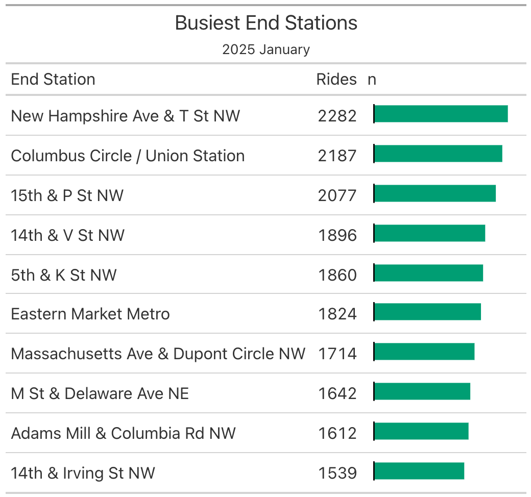

The figure is very similar to the above table. It has an additional column, next to the rides column showing the number of rides as a horizontal bar. The fewer the number of rides, the shorter the bar. — Table 8.4: A table with a bar plot visualization of count of rides

Even though we have written the code for the final table in Table 8.4 in multiple code chunks to demonstrate each step, one at a time, in a real data science workflow we would have written the code in fewer chunks even if we had written progressively checking it at each step.

A clean workflow might potentially have three main parts: one for importing the raw data, the second one for getting the summary data ready for the table, and the third one for getting a publication ready table. The full code would look like

# Part 1 Getting Data Ready
bikes <-
  read_csv(
  here::here("data", "202501-capitalbikeshare-tripdata.csv")
) 

glimpse(bikes)

# Part 2 - Getting Summary Data Ready for the Table

bikes_table <- bikes |> 
  drop_na(end_station_name) |>
  count(end_station_name) |>
  slice_max(order_by = n, n = 10)

# Part 3 - Create and Make the Table Pretty

bikes_table |> 
  gt() |> 
  cols_label(
    end_station_name = "End Station",
    n = "Rides"
  ) |> 
  tab_header(
    title = "Busiest End Stations",
    subtitle = "2025 January"
  ) |> 
  gt_plt_bar(
    column = n,
    color = "#009E73",      
    keep_column = TRUE
  )

This all looks great and the code gave us what we wanted. However, we still have a challenge remaining: we only did this table for January 2025. What if we had to do this for all the other months in 2025 as well? February 2025 for instance? If you are thinking of copying and pasting the above code and then changing the dataset that is being read in and the subtitle to “2025 February”, then we have some news for you. Copying and pasting is not sustainable in the long term and is error-prone. Hence, instead, we will learn about functions and iterations to make our solution easy to use for any month in 2025.

8.3 Functions

To automate the process of making tables for any month in 2025, we will first take a detour and learn about functions. We first introduced the idea of a function in Section 1.1. There are two types of functions: 1) functions that are already built into R or a package that you install, such as the ones you have been using all this time, and 2) functions that the user creates. And now, it is time to learn to write your own functions.

Let’s start with the simplest possible function: one that simply says “hello” when called.

print_hello <- function(){
  print("hello")
}

Now that we have a function defined as print_hello() we can go ahead and use it.

print_hello()

[1] "hello"

It did indeed print hello. Let’s understand the overall structure of functions.

function_name <- function() {
  do_something
}

Function definitions include a function_name which is essentially the name we give it so that you can call it later. Since a function is used to do some action then using action verbs for function names makes sense. The function() part of the code tells R that you are creating a new function. Between the curly braces { } lies the “body” of the function. Everything inside these braces runs when the function is called.

The print_hello() function we just made is a bit boring because it does the exact same thing every single time. Imagine you wanted to greet specific people instead. Without a flexible function, your code would quickly look like this repetitive mess:

print("hello Isabella")
print("hello Andrew")
print("hello Nihan")

If you look closely at those three lines, you’ll see a clear pattern. There is a fixed part (“hello”) and a blank space that changes depending on who you are talking to:

print("hello ❏")
print("hello ❏")
print("hello ❏")

In programming, we can use a placeholder variable for that empty box:

print("hello a person")
print("hello a person")
print("hello a person")

To make our function handle this, we can introduce an argument (a variable placeholder) inside the function() definition. We will call our placeholder person, and use paste() to glue “hello” and the person’s name together.

print_hello <- function(person){
  print(paste("hello", person))
}

We can now pass different names into the person argument:

print_hello("Isabella")

[1] "hello Isabella"

print_hello("Andrew")

[1] "hello Andrew"

print_hello("Nihan")

[1] "hello Nihan"

You can also explicitly name the argument when you call the function, which makes your code much easier to read:

print_hello(person = "Isabella")

[1] "hello Isabella"

Whenever you need a function to accept a variable input from the user, you use this updated pattern:

function_name <- function(argument) {
  do_something(argument)
}

function_name(argument = argument_value)

What if you need your function to take more than one piece of information? For example, what if you want to greet two people at the same time?

Without a function, your copy-pasted code would look like this:

print("hello Isabella and Mateo")
print("hello Andrew and Lakshimi")
print("hello Nihan and Selin")

Once again, let’s identify the patterns and find the “empty boxes” that change each time:

print("hello ❏ and ❍")
print("hello ❏ and ❍")
print("hello ❏ and ❍")

We have two distinct placeholders here:

print("hello a person and another person")
print("hello a person and another person")
print("hello a person and another person")

To handle multiple placeholders, we simply separate our arguments with a comma inside the function() definition. Let’s rewrite print_hello() to accept both person1 and person2 as arguments.

print_hello <- function(person1, person2){
  print(paste("hello", person1, "and", person2))
}

Now, when you call the function, you must provide values for both placeholders. You can do this implicitly by matching the order of the arguments:

print_hello("Isabella", "Mateo")

[1] "hello Isabella and Mateo"

Or, even better, you can explicitly name them to ensure they go into the right “boxes”, regardless of order:

print_hello(person1 = "Isabella", person2 = "Mateo")

[1] "hello Isabella and Mateo"

Whenever you need a function to accept multiple inputs from the user, the body of the function does something to both of the arguments:

function_name <- function(argument1, argument2) {
  do_something(argument1, argument2)
}

function_name(argument1 = argument1_value, argument2 = argument2_value)

Now that you know how to build a function with multiple arguments, we can apply this exact logic to automate our 2025 tables, using the specific month we want as our argument.

Before we wrap our table-making pipeline into a function, let’s look at the raw code we’ve been using. Just like before, we want to look for the parts of the code that need to change every time we want to generate a table for a new month. Take a look at the template below. Can you spot the empty boxes (❏ and ❍)?

# Part 1 Getting Data Ready
bikes <-
  read_csv(
  here::here(
1    "data", "❏"
  )
) 
# Part 2 - Getting Summary Data Ready for the Table

bikes_table <- bikes |> 
  drop_na(end_station_name) |>
  count(end_station_name) |>
  slice_max(order_by = n, n = 10)

# Part 3 - Creating and Making the Table Pretty

bikes_table |> 
  gt() |> 
  cols_label(
    end_station_name = "End Station",
    n = "Rides"
  ) |> 
  tab_header(
    title = "Busiest End Stations",
2    subtitle = "2025 ❍"
  ) |> 
  gt_plt_bar(
    column = n,
    color = "#009E73",      
    keep_column = TRUE
  )

1: For each month, we need to specify the csv file that is read.
2: For each month, we need to specify the subtitle of the table based on the month label (i.e., January, February etc.).

If we want to run this for January, the first box (❏) needs to be the file name "202501-capitalbikeshare-tripdata.csv", and the second box (❍) needs to be the subtitle label "January" as we have done. Instead of copying, pasting, and manually changing these strings for all 12 months, we can create a single argument called month and let R do the heavy lifting. At a first glance, it might seem like, we have two boxes, and we need two separate arguments. However, that is not true. Both of these boxes depend on the month so all we need to get from the user in order to compile the table is the month.

Let’s start defining our function make_bike_table() with its single argument: month.

make_bike_table <- function(month){
}

Let’s assume the user enters the month as a number between 1 - 12.

month <- 1

Before building our function’s body, let’s work on the boxes outside of the function first. We can use lubridate::ymd() to dynamically build a temporary date object. By anchoring our input to a real date, it will be easier to switch between “01” and “January” labels moving forward. Here, the day is to be the first of the month but that’s really irrelevant since we will never use the day of the month in our analysis.

date_obj <- ymd(paste("2025", month, "01"))
date_obj

[1] "2025-01-01"

Now that R recognizes the date, we can safely extract our two different required formats. First, we need a two-digit numeric string for our file path. We extract the numeric month and use stringr::str_pad() to ensure it always has a leading zero if it’s a single digit.

month_numeric <- str_pad(month(date_obj), width = 2, pad = "0") 
month_numeric

[1] "01"

Second, we need the full text name of the month for our table’s subtitle. We can use lubridate::month() with label = TRUE and abbr = FALSE to pull the full word.

month_name <- as.character(month(date_obj, label = TRUE, abbr = FALSE)) 
month_name

[1] "January"

With our two formats saved into variables, we can dynamically build our text strings. For the dataset, we want to target a file named exactly like this:

"202501-capitalbikeshare-tripdata.csv"

[1] "202501-capitalbikeshare-tripdata.csv"

Using str_c(), we can exchange the fixed month text for our dynamic month_numeric variable:

str_c("2025", month_numeric, "-capitalbikeshare-tripdata.csv")

[1] "202501-capitalbikeshare-tripdata.csv"

Let’s save this dynamic path into a variable called file_name so that we can use it later on.

file_name <- str_c("2025", month_numeric, "-capitalbikeshare-tripdata.csv")

We can do the exact same thing for our table’s subtitle, gluing the year to our textual month_name:

str_c("2025", month_name, sep = " ")

[1] "2025 January"

Now, let’s put it all together to define the body and complete the function.

make_bike_table <- function(month) {
  
  # 1. Standardize the input into an R date object
  date_obj <- ymd(str_c("2025", month, "01", sep = " "))
  
  # 2. Extract the two formats we need
  month_numeric <- str_pad(month(date_obj), width = 2, pad = "0")              
  month_name <- as.character(month(date_obj, label = TRUE, abbr = FALSE))   
  
  # Part 1: Getting Data Ready
  file_name <- str_c("2025", month_numeric, "-capitalbikeshare-tripdata.csv")
  
  bikes <- read_csv(
    here::here("data", file_name)
  ) 
  
  # Part 2: Getting Summary Data Ready for the Table
  bikes_table <- bikes |> 
    drop_na(end_station_name) |>
    count(end_station_name) |>
    slice_max(order_by = n, n = 10)
  
  # Part 3: Creating the Beautiful Table
  bikes_table <-
    bikes_table |> 
    gt() |> 
    cols_label(
      end_station_name = "End Station",
      n = "Rides"
    ) |> 
    tab_header(
      title = "Busiest End Stations",
      subtitle = str_c("2025", month_name, sep = " ")
    ) |> 
    gt_plt_bar(
      column = n,
      color = "#009E73",      
      keep_column = TRUE
    )
bikes_table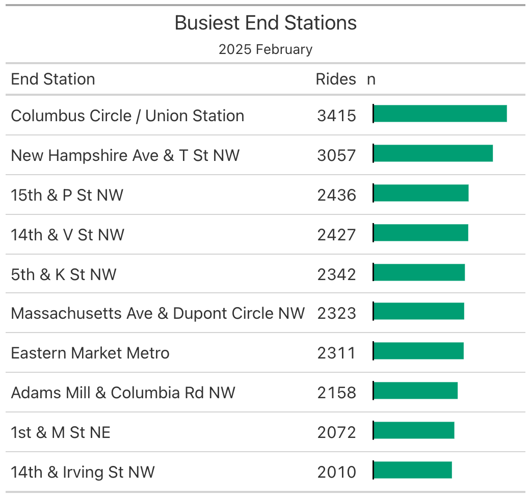
}

1make_bike_table(month = 2)

1: We can use our completed function make_bike_table() with the month argument set to 2. In Table 8.5 we can see the summary table for the month of February 2025.

The table is very similar to the above table. Now the subtitle reads 2025 February and the end stations with high number of rides are now different. — Table 8.5: A table with a bar plot visualization of count of rides for the month of February

Always build the body of your function outside of the function first. When writing functions, do not start writing your code inside the curly braces {} first. Instead, test things first outside the function. For instance, in our bike table example, we first made sure date_obj, month_numeric, month_name, and file_name all work with an arbitrary argument assignment (e.g., we tested with month of January by setting month <- 1). Once we were sure to see things working outside of the function, then we put these variables inside the function.

8.4 Iterations

Now that our make_bike_table() function is built and working beautifully, we can easily generate a table for any month we want. But what if we want to generate the tables for the entire year?

We could copy and paste the function 12 times, changing the input manually each time:

make_bike_table(1)
make_bike_table(2)
.
.
.
make_bike_table(11)
make_bike_table(12)

But this brings us right back to our original problem: unnecessary repetition. If you find yourself copying and pasting the exact same line of code more than twice, it is a clear sign that you can do better.

Follow the “Rule of three” (Fowler 2018). If you catch yourself writing and copying and pasting code the third time, you should find a computational solution (e.g., factors and iteration) to avoid duplication.

Iteration is used whenever there is a repeating action across a different set of values or items. We can tell R to go through a sequence of items and do the action for each item in the sequence. In R, for loops are one of the most fundamental ways of iterating.

Let’s look at a very basic for loop to see how it works. This loop steps through the numbers 1 to 5 and prints them one by one:

for(i in 1:5){
  print(i)
}

[1] 1
[1] 2
[1] 3
[1] 4
[1] 5

In this code, i acts as a temporary placeholder variable (often called a loop index). The first time through the loop, i is equal to 1. The second time, i becomes 2, and so on, until it reaches 5. At each step of the loop, the value of i at that step is printed.

You don’t have to use numbers, and you don’t have to use the index i. You can loop through a vector of text strings, and name your placeholder variable anything that makes sense for your data:

for(fruit in c("Apples", "Oranges", "Bananas")){
  print(fruit)
}

[1] "Apples"
[1] "Oranges"
[1] "Bananas"

for (k in c(3, 8, 10)) {
  print(k * 2)
}

What value does the variable k hold during the second pass of the loop?
How many times will the body of this loop execute?
What will be the output of this code?

Check footnote for answer¹

Before we create a loop for the bikes table example in the previous sections, let’s look at two other practical examples to see how loops can accumulate values or transform existing data.

Example 1: Cumulative Running Total (The Piggy Bank)

Imagine you are saving money, adding an increasing amount to your piggy bank every day ($1 on day one, $2 on day two, and so on). We can use a loop to track your total savings over 10 days by adding the current day’s number to a running total.

1days <- 10

2total_savings <- 0

3for (day in 1:days) {
4  total_savings <- total_savings + day
5  print(stringr::str_c(
    "Day ", day, ": Total saved is $", total_savings
  ))
}

1: We start buy setting the number of days to be 10.
2: We initialize our total savings tracker at 0.
3: Our for loop index is going to be day. The for loop will go through setting day equal to 1, 2, 3, ….10.
4: At each pass of the loop (i.e., on each day) we add the current day’s amount to our total savings.
5: We print the process on each pass of the loop (i.e., for each day). If strings are not your favorite part of data science, feel free to just print(total_savings).

[1] "Day 1: Total saved is $1"
[1] "Day 2: Total saved is $3"
[1] "Day 3: Total saved is $6"
[1] "Day 4: Total saved is $10"
[1] "Day 5: Total saved is $15"
[1] "Day 6: Total saved is $21"
[1] "Day 7: Total saved is $28"
[1] "Day 8: Total saved is $36"
[1] "Day 9: Total saved is $45"
[1] "Day 10: Total saved is $55"

Example 2: Converting Units (Fahrenheit to Celsius)

Suppose we have a vector of temperature readings in degrees Fahrenheit, and we want to convert every single one of them to degrees Celsius. We can use a for loop to step through each position (i) of our vector, apply our math formula, and save the result into a new vector.

1fahrenheit_temps <- c(32, 50, 68, 86, 104)

2celsius_temps <- numeric(length(fahrenheit_temps))

3for (i in 1:length(fahrenheit_temps)) {
4  celsius_temps[i] <- (fahrenheit_temps[i] - 32) * 5 / 9
}


5data.frame(Fahrenheit = fahrenheit_temps, Celsius = celsius_temps)

1: We start by defining a vector of Fahrenheit temperatures called fahrenheit_temps, which we will convert to Celsius.
2: We create an empty numeric vector called celsius_temps for Celsius temperatures. Currently, it is empty because we have not yet calculated the Celsius equivalents. Even though it is empty, it has the exact same length as fahrenheit_temps.
3: The for loop will have an index of i. The i index will start at 1 and will go all the way up to 5 which is the length of fahrenheit_temps vector.
4: For each step in the loop we will use the Fahrenheit to Celsius conversion formula. For instance, in the first step, i will be set to 1 and celsius_temps[i] will be celsius_temps[1], which means the first element of the celsius_temps vector will equal to the first element of the fahrenheit_temps vector, minus 32, and this difference is then multiplied by 5/9.
5: In this step, we take the five elements of fahrenheit_temps and celsius_temps and display them side-by-side in a data frame.

  Fahrenheit Celsius
1         32       0
2         50      10
3         68      20
4         86      30
5        104      40

Now that you understand how a for loop works, we can go back to the bikes table example and completely eliminate the copy-pasted function lines from the beginning of this section.

We will tell R to loop through the numbers 1 to 12 for each month of 2025. Then, inside the loop, the index i will represent the current month number, which we pass directly into our make_bike_table() function.

When running a function inside a loop, R will execute the code but won’t automatically print the resulting visual tables to your screen. To force R to display each table as it generates them, we wrap our function call inside print().

for(i in 1:12){
  print(make_bike_table(i))
}

Because of space reasons, we did not print 12 tables here, but you should see them on your end when you run the code for this chapter.

1.) The first, second, and third passes will have values of k set to 3, 8, and 10 respectively so the second pass will set k as 8. 2.) Three times, 3.) 6, 16, 20, each value of k is multiplied by 2 at each pass.↩︎