7Dealing with Datasets: Joining, Pivoting, and Importing Datasets
At this point, you know a lot about dealing within a given dataset. You have learned how to explore it to determine how many variables and observations it has and how variables are stored. And for such variables, you have learned how to clean them, visualize them, and summarize them numerically. Now, it is time for us to shift our attention to datasets themselves.
Merge multiple datasets using joins
Convert datasets between long and wide formats
Import external datasets into R
7.1 Joining Datasets
Up until now, every time we analyzed data, we loaded a single data frame. It’s easy to get the impression that all data in the wild lives in one neat, isolated file. In the real world, it almost never does. Instead, data is usually stored in a database, which is a collection of multiple tables that are connected to one another. Think of it like a massive spiderweb of data frames. Organizations split their data into different tables to keep things organized, secure, and efficient.
For instance, in a database of a hospital, one dataset might hold patient contact info and insurance data. A separate dataset tracks daily doctor visits, and a third table lists prescriptions. The hospital doesn’t cram all of this into one giant file because a patient might have dozens of visits or prescriptions over time, and repeating their home address multiple times would be messy and slow down the system.
As a data scientist, you will be working often on projects that deal with multiple datasets, and combining them as one data frame becomes part of the process of analyzing the data. In this section, we explore various methods of merging datasets as one.
7.1.1 Data Context
Football, commonly known as soccer in the United States, is the most popular sport around the world with over 3.5 billion fans (Singh 2025). When this chapter was first released, the FIFA (International Federation of Association Football) Men’s Football World Cup 2026 was about to take place. Hence, we wanted to work with a few datasets containing information about some of the teams that qualified for the tournament, including the association they belong to, their world ranking, and the capital city of their corresponding country, among other information. For simplicity, the datasets will be small so that we can easily illustrate the process of joining them. You will get to practice joining more realistic and larger datasets in Exercises.
Let us go ahead and load the packages we will use in this chapter. All the join functions that we will use come from the {dplyr} package, which loads along with other tidyverse packages when library(tidyverse) is called.
library(tidyverse)
── Attaching core tidyverse packages ──────────────────────── tidyverse 2.0.0 ──
✔ dplyr     1.2.1     ✔ readr     2.2.0
✔ forcats   1.0.1     ✔ stringr   1.6.0
✔ ggplot2   4.0.3     ✔ tibble    3.3.1
✔ lubridate 1.9.5     ✔ tidyr     1.3.2
✔ purrr     1.2.2
── Conflicts ────────────────────────────────────────── tidyverse_conflicts() ──
✖ dplyr::filter() masks stats::filter()
✖ dplyr::lag()    masks stats::lag()
ℹ Use the conflicted package (<http://conflicted.r-lib.org/>) to force all conflicts to become errors
library(hellodatascience)
We will also load the datasets country_rank, country_capital, and confederations provided in the {hellodatascience} package.
Now we can run the name for each of the datasets and look at the documentation to get familiar with each of them.
country_rank
# A tibble: 7 × 3
  country       fifa_rank confederation
  <chr>             <dbl> <chr>
1 United States        16 CONCACAF
2 Mexico               15 CONCACAF
3 Japan                18 AFC
4 Ghana                74 CAF
5 Ecuador              23 CONMEBOL
6 New Zealand          85 OFC
7 Spain                 2 UEFA
The country_rank dataset has information on 7 teams and 3 variables. The variables represented in each column of the data are shown in Table 7.1.
Table 7.1: Documentation of variables in the country_rank dataset
Variable Name
Description
country
name of the country men’s soccer team participating in the World Cup 2026
fifa_rank
FIFA world ranking as of April, 2026
confederation
region/continent association affiliated to FIFA
country_capital
# A tibble: 5 × 3
  country  capital     population
  <chr>    <chr>            <dbl>
1 Mexico   Mexico City      132.
2 Japan    Tokyo            123.
3 Ghana    Accra             34.4
4 Colombia Bogota            53.4
5 Spain    Madrid            47.9
The country_capital dataset has information on 5 countries and 3 variables. The variables represented in each column of the data are shown in Table 7.2.
Table 7.2: Documentation of variables in the country_capital dataset
Variable Name
Description
country
name of the country
capital
name of the country’s capital city
population
population size of the country in millions in 2025
confederations
# A tibble: 7 × 2
  confederation region
  <chr>         <chr>
1 AFC           Asia and Australia
2 CAF           Africa
3 CONCACAF      North & Central America and the Caribean
4 CONMEBOL      South America
5 OFC           Oceania
6 UEFA          Europe
7 FIFA          World
And lastly, the confederations dataset has information on the 7 confederations, including FIFA, and 2 variables. The variables represented in each column of the data are shown in Table 7.3.
Table 7.3: Documentation of variables in the confederations dataset
Variable Name
Description
confederation
name of the FIFA member association
region
region or continent overseed by the confederation
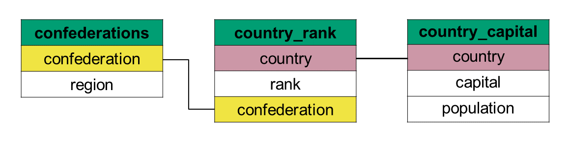
When you are working with multiple datasets from a single database, your first step is understanding how those separate datasets connect to one another. A great way to do this is by looking at the relations between datasets, like the one shown in Figure 7.1. This diagram acts as a visual map of the entire database. It allows you to see all the available data frames at a glance, the variables inside them, and—most importantly—the key variables that act as the connectors of two data frames.
Let’s look at how this works using the datasets shown in Figure 7.1:
Connecting by country: If you want to combine the country_rank and country_capital datasets, the figure shows that country is the matching key variable present in both tables.
Connecting by confederation: On the other hand, if you want to link the country_rank dataset with the confederations dataset, you would use the confederation variable to match.
Figure 7.1: Diagram showing the relationship between datasets
Once we have identified a connecting key, we have to determine how we want to join our data frames. In {dplyr}, there are two main types of joins: mutating joins and filtering joins.
Mutating Joins (Adding Information): Think of the word mutate as “adding new columns.” A mutating join matches up rows from two tables using a key, and then adds new columns of information from the second data frame onto the first.
Filtering Joins (Cleaning Rows): Think of the word filter as “keeping or removing rows.” A filtering join doesn’t add any new columns at all. Instead, it looks at the second data frame and uses it as a checklist to keep or drop rows in your first table.
7.1.2 Mutating Joins
All mutating joins add new variables (i.e., columns) from a secondary dataset to a primary dataset. However, they differ in how they handle rows that don’t find a matching partner. Depending on your goal, you will choose between a left join, a right join, a full join, or an inner join.
The left join is one of the most common of data joins. You use a left join whenever you have a primary dataset (the “left” data frame) and you want to pull in additional variables from a secondary dataset (the “right” data frame), without losing any of your original observations in the left data frame.
Imagine you want to look at the country_rank dataset, keep all its original information, but add a new column showing the geographical region that each football confederation represents from the country_capital dataset. In left_join(x, y), x is our primary data frame and y is our secondary data frame:
Since this is a left_join() the primary dataset will be the country_rank. All the columns and rows of the country_rank will be in the final merged dataset.
2
The secondary dataset is country_capital. Its additional columns (capital and population) will be added to the final dataset, but only for the countries that already exist in the primary dataset. In other words, only matching rows get these new columns filled in.
3
Even though by is the third argument, it is the first thing you should think about! This is the key variable R uses to line up the rows between the two datasets.
# A tibble: 7 × 5
  country       fifa_rank confederation capital     population
  <chr>             <dbl> <chr>         <chr>            <dbl>
1 United States        16 CONCACAF      <NA>              NA
2 Mexico               15 CONCACAF      Mexico City      132.
3 Japan                18 AFC           Tokyo            123.
4 Ghana                74 CAF           Accra             34.4
5 Ecuador              23 CONMEBOL      <NA>              NA
6 New Zealand          85 OFC           <NA>              NA
7 Spain                 2 UEFA          Madrid            47.9
When you look at the resulting data frame, pay close attention to how the unmatched rows were handled:
The NA values: The United States, Ecuador, and New Zealand all have NA (missing values) for capital and population. Because a left join insists on keeping every row from the primary dataset, (country_rank) R fills in these columns with NA when it can’t find a matching country in country_capital.
The dropped rows: Colombia was present in the original country_capital dataset, but it is completely missing from our final merged table because country_capital is the secondary (right) data frame. In a left join, rows from the right data frame that fail to match the left table are automatically dropped.
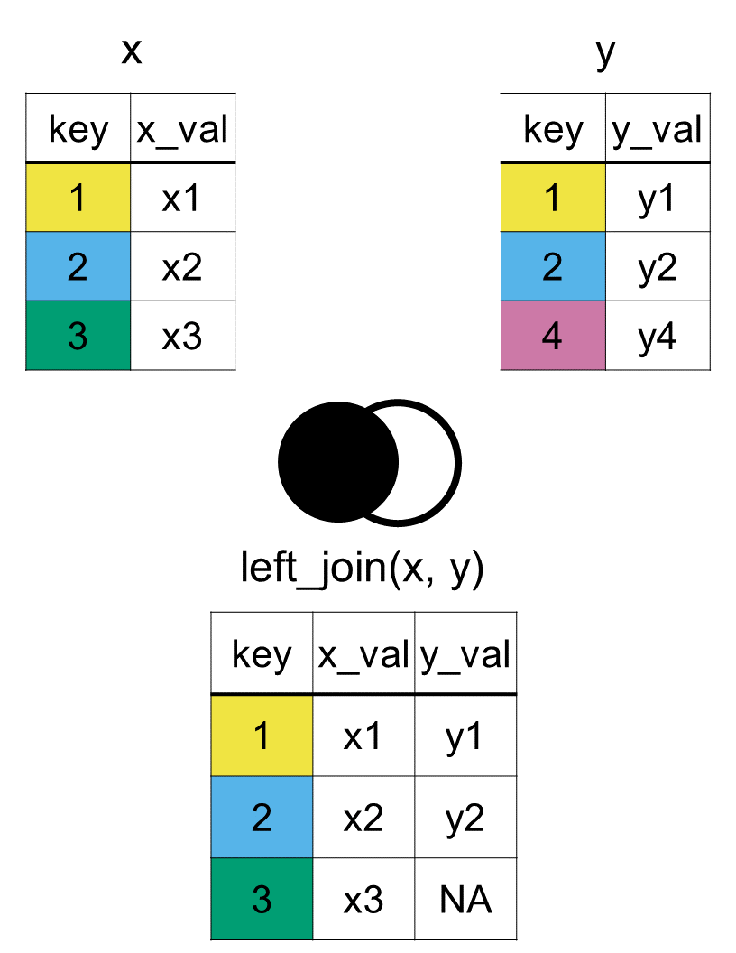
In general, as shown in Figure 7.2, the output from a left join using the left_join(x, y, by = "key") function will include all rows from x, but only keep the matching ones from y and will include all columns from both x and y.
Figure 7.2: Diagram of the resulting dataset from a left join of datasets x and y
Did you notice that there is no connecting key between the country_capital and confederations datasets? This means we cannot merge just the two of them. However, we can join them by first merging one of the datasets to country_rank, then join the other dataset such as follows:
left_join(x = country_rank, y = country_capital, by ="country") |>left_join(y = confederations, by ="confederation")
# A tibble: 7 × 6
  country       fifa_rank confederation capital     population region
  <chr>             <dbl> <chr>         <chr>            <dbl> <chr>
1 United States        16 CONCACAF      <NA>              NA   North & Central …
2 Mexico               15 CONCACAF      Mexico City      132.  North & Central …
3 Japan                18 AFC           Tokyo            123.  Asia and Austral…
4 Ghana                74 CAF           Accra             34.4 Africa
5 Ecuador              23 CONMEBOL      <NA>              NA   South America
6 New Zealand          85 OFC           <NA>              NA   Oceania
7 Spain                 2 UEFA          Madrid            47.9 Europe
The resulting data frame contains all the variables from all the data sets in the order that we joined them. Missing values were filled in with NA. In the first left join, Colombia was dropped since it was unmatched and then in the second left join, FIFA was dropped since it was also unmatched. Even though Colombia and FIFA exist in the database, they do not appear in this particular merged dataset.
If there is a left join, is there a right join too? Of course, a right join is another type of mutating join, which combines columns from two data sets into one. But then how would a right join differ from a left join?
As you might guess from the name, a right join completely flips the priority. In right_join(x, y), the secondary dataset y (the “right” data frame) becomes the primary focus. The final merged dataset will keep every single row from the right data frame and will drop rows from the left data frame if they don’t find a match.
Let’s see what happens when we use a right join on our datasets:
In a right_join(), the dataset passed to x (country_rank) is now the secondary dataset. Rows from this data frame will be dropped if they don’t match the right data frame.
2
The dataset passed to y (country_capital) is the primary dataset. Every single row and column from this table will appear in the final output.
3
Just like before, by specifies the key variable (country) used to match the datasets together.
# A tibble: 5 × 5
  country  fifa_rank confederation capital     population
  <chr>        <dbl> <chr>         <chr>            <dbl>
1 Mexico          15 CONCACAF      Mexico City      132.
2 Japan           18 AFC           Tokyo            123.
3 Ghana           74 CAF           Accra             34.4
4 Spain            2 UEFA          Madrid            47.9
5 Colombia        NA <NA>          Bogota            53.4
Colombia is now included in the final dataset! Because country_capital is on the right, R insists on keeping it, filling in its missing rank and confederation columns with NA because Colombia wasn’t in the country_rank table. The United States, Ecuador, and New Zealand have completely vanished from the final dataset. Since they didn’t exist in the primary right table (country_capital), they were dropped.
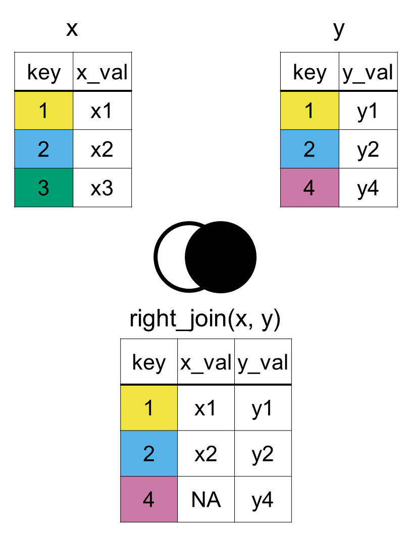
In conclusion, a right join, using the right_join(x, y, by = "key") function, will include all rows from y, and only the matching ones form x as seen in Figure 7.3. All the columns from both the datasets will be included.
Figure 7.3: Diagram of the resulting dataset from a right join of datasets x and y
What would happen if we do a right join with country_rank and country_capital, but we reverse the order of the dataset in the arguments?
right_join(x = country_capital, y = country_rank, by ="country")
Both left and right joins have a habit of leaving some observations (i.e., rows) behind. A left join drops unmatched rows from the right dataset, and a right join drops unmatched rows from the left dataset.
But what if you don’t want to lose any data? If your goal is to preserve every single row from both datasets, you use a full join with the full_join() function.
# A tibble: 8 × 5
  country       fifa_rank confederation capital     population
  <chr>             <dbl> <chr>         <chr>            <dbl>
1 United States        16 CONCACAF      <NA>              NA
2 Mexico               15 CONCACAF      Mexico City      132.
3 Japan                18 AFC           Tokyo            123.
4 Ghana                74 CAF           Accra             34.4
5 Ecuador              23 CONMEBOL      <NA>              NA
6 New Zealand          85 OFC           <NA>              NA
7 Spain                 2 UEFA          Madrid            47.9
8 Colombia             NA <NA>          Bogota            53.4
We can see all countries (i.e., all rows) from both datasets regardless if there is a match or not. Variables in unmatched rows are filled in with blank values of NAs.
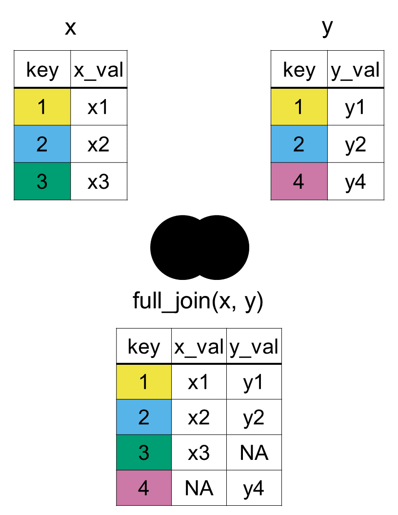
Simply, a full join with the function full_join(x, y, by = "key") will include all rows that are in xory and all the columns in both x and y. In Figure 7.4, we can see that the output starts with all rows from x, followed by the remaining unmatched y rows.
Figure 7.4: Diagram of the resulting dataset from a full join of datasets x and y
When learning joins, it is tempting to always use full_join() to avoid accidentally losing data. However, good data science requires choosing the join that yields the optimal number of rows and columns for your specific analysis. Always defaulting to a full join can ruin your workflow by introducing massive NA bloat with hundreds of irrelevant, empty rows that you do not actually need. Always ask yourself what your primary dataset is before writing your join code.
How would we join the datasets if we wanted the resulting data frame to keep all rows, but have the variables in this particular order: country, capital, population, fifa_rank, confederation, and region?
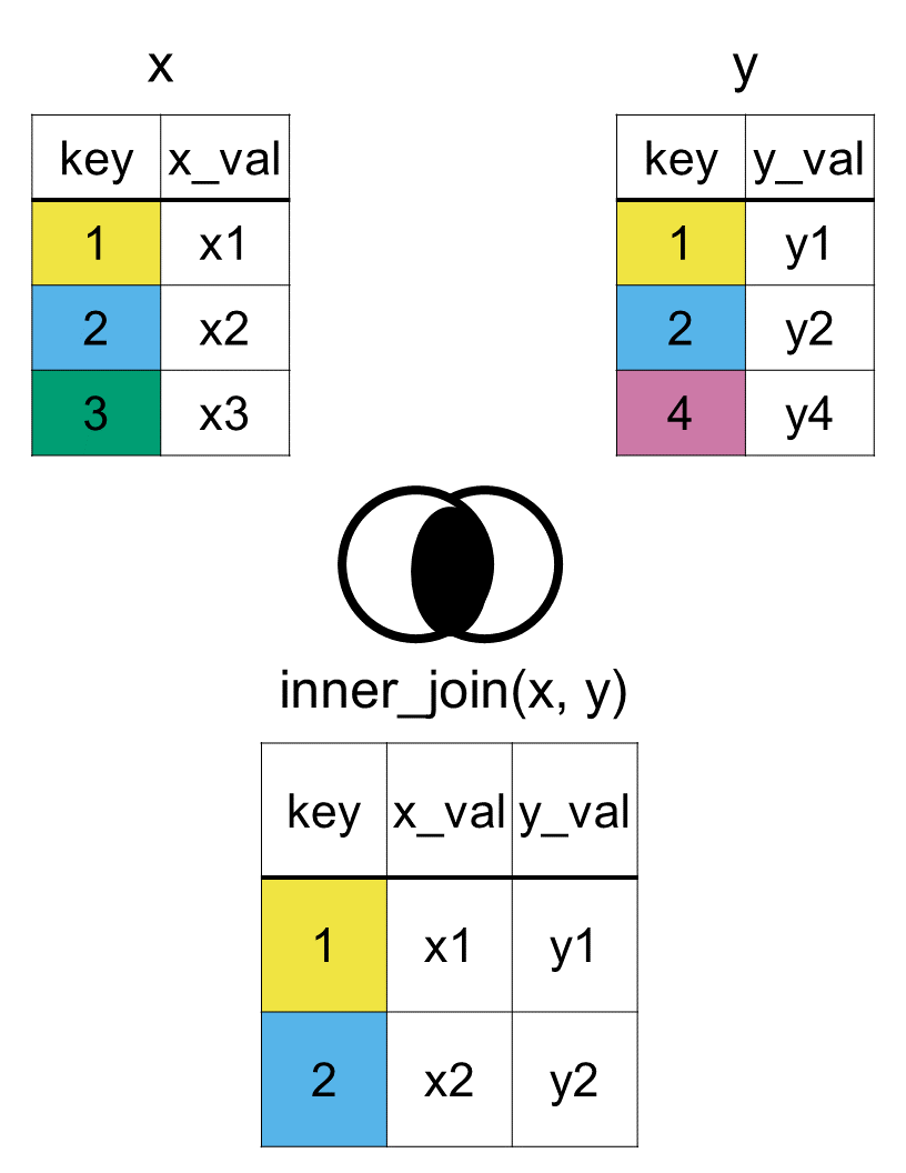
The last type of mutating join combines the columns of two datasets, but only keeps the matching rows, the inner join.
Let us see what rows are kept when we do an inner join between country_rank and country_capital.
inner_join(x = country_rank, y = country_capital, by ="country")
# A tibble: 4 × 5
  country fifa_rank confederation capital     population
  <chr>       <dbl> <chr>         <chr>            <dbl>
1 Mexico         15 CONCACAF      Mexico City      132.
2 Japan          18 AFC           Tokyo            123.
3 Ghana          74 CAF           Accra             34.4
4 Spain           2 UEFA          Madrid            47.9
The rows corresponding to the United States, Ecuador, and New Zealand in country_rank were dropped. The row for Colombia in country_capital was also not included.
Hence an inner join, computed using the function inner_join(x, y, by = "key"), keeps the observations (rows) that are in both xandy identified by the key. The most important property of an inner join is that unmatched rows are not included in the result. This join keeps intersecting rows, similar to intersecting sets in a Venn diagram as we can see in Figure 7.5 below.
Figure 7.5: Diagram of the resulting dataset from an inner join of datasets x and y
As we saw from all the examples, the main purpose of mutating joins: left, right, full, inner, is to allow you to combine variables (columns) from two data frames by first matching observations by their keys, then adding variables (columns) from the second data frame to the right of the variables of first data frame. The total number of columns will increase, but the number of observations (rows) may either increase, decrease, or stay the same, depending on the type of mutating join we use.
7.1.3 Filtering Joins
At the end of section Section 7.1.1 we also introduced filtering joins. Recall, a filtering join filters (keeps or deletes) the rows in a data frame that do not have a matching key value in another data frame.
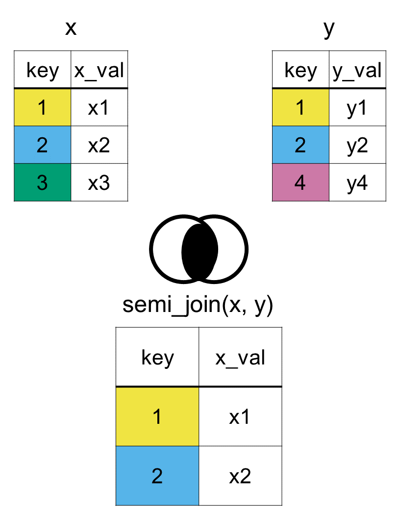
A semi join is a popular type of filtering join. If we do a semi join with country_rank and country_capital we get the following data frame.
semi_join(x = country_rank, y = country_capital, by ="country")
# A tibble: 4 × 3
  country fifa_rank confederation
  <chr>       <dbl> <chr>
1 Mexico         15 CONCACAF
2 Japan          18 AFC
3 Ghana          74 CAF
4 Spain           2 UEFA
We only include the variables (columns) and observations (rows) from country_rank. The United States, Ecuador, and New Zealand in country_rank did not have a match in country_capital and were dropped. The dataset country_capital determined which rows to keep from country_rank. In a way the final dataset has the country_rank information for countries for which we have information on capitals.
A semi join is similar to an inner join in that they keep only matching rows, with the difference that a semi join does not include variables from the second dataset.
A semi join, using the function semi_join(x, y, by = "key"), would allow us to keep rows in x that match in y and only keep the columns of x, as seen in Figure 7.6.
Figure 7.6: Diagram of the resulting dataset from a semi join of datasets x and y
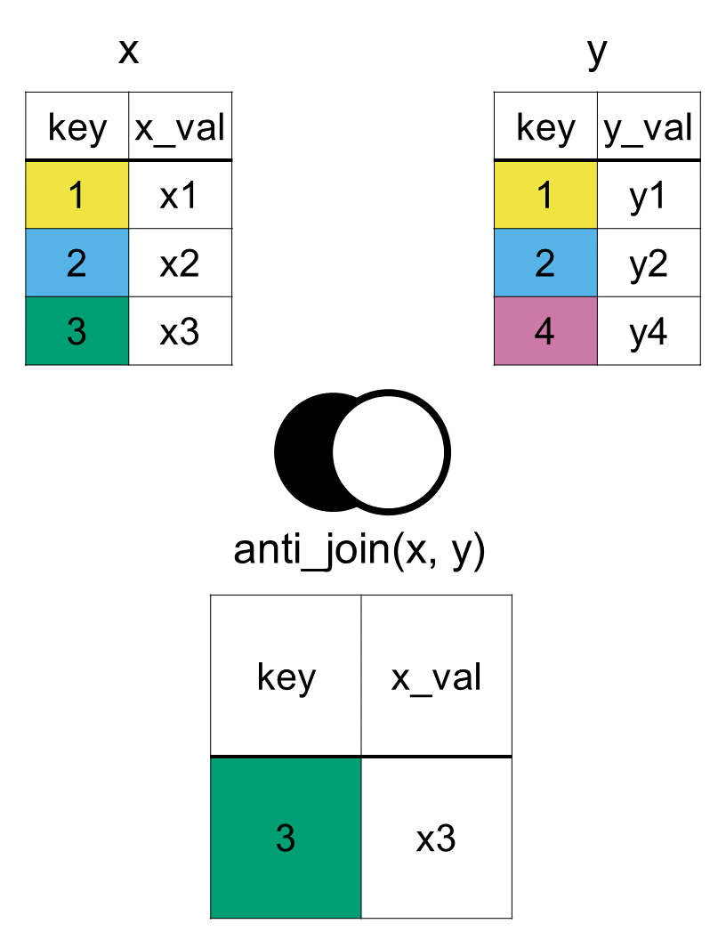
The opposite of a semi join is an anti join. While a semi join keeps rows that do find a match, an anti join does the exact opposite: it keeps rows from your primary dataset that do not have a matching partner in the secondary dataset.
anti_join(x = country_rank, y = country_capital, by ="country")
# A tibble: 3 × 3
  country       fifa_rank confederation
  <chr>             <dbl> <chr>
1 United States        16 CONCACAF
2 Ecuador              23 CONMEBOL
3 New Zealand          85 OFC
The final output only contains the original variables from country_rank. Just like a semi join, a filtering join never adds new columns. The only rows kept are the United States, Ecuador, and New Zealand. Because these three countries do not exist in country_capital, they are the only ones that pass through the filter.
An anti join, using the function anti_join(x, y, by = "key"), is also a filtering join, but it would keep observations in x that do not have a match in y, as we can see in Figure 7.7 below. A common use of it is to check for rows in x that do not have a match in y, in preparation for joining two datasets with a mutating join.
Figure 7.7: Diagram of the resulting dataset from an anti join of datasets x and y
7.1.4 A Summary of Joins
Regardless of which type of join you decide to do, all join functions have the same general format of something_join(x, y, by = "key"), where x represents the first data frame, y represents the second data frame, and key is the variable that the two frames are connected by.
Join functions take a pair of data frames (x and y) and return a data frame.
The order of the rows and columns in the output is primarily determined by x.
The rows and columns that are kept depend on the type of join you do.
The information in Table 7.4 shows us the rows and columns from x and y that are kept in the resulting merged dataset.
Table 7.4: A summary of dplyr’s join functions in the format of something_join(x, y)
Join function
Rows from x
Columns from x
Rows from y
Columns from y
left_join()
all
all
matched
all
right_join()
matched
all
all
all
full_join()
all
all
all
all
inner_join()
matched
all
matched
all
semi_join()
matched
all
none
none
anti_join()
unmatched
all
none
none
7.2 Pivoting Data Between Wide and Long Formats
Datasets come in various structures, meaning that data can be organized in different ways. Sometimes the way the data frame is presented is not ideal for our analysis and we need to pivot it in a different way. In tidyverse (specifically {tidyr}), pivoting refers to reshaping a data frame so that it is either:
longer: more rows, fewer columns, or
wider: fewer rows, more columns.
Pivoting does not change the underlying data, only how the data is organized. Ideally, we want a dataset to be tidy, which means that every row is an observation and every column represents a variable. Functions in the {tidyverse} packages require data frames to be tidy. Unfortunately, that is not always the case.
7.2.1 Pivot Longer
Let’s say we were given the following data on participation ranking for Mexico and the United States for the last four World Cups.
mx_us_wc_ranks
# A tibble: 2 × 5
  country       `2010` `2014` `2018` `2022`
  <chr>          <dbl>  <dbl>  <dbl>  <dbl>
1 Mexico            14     10     12     22
2 United States     12     15     NA     14
The data is presented in a way that each year is its own variable (column) and rankings are spread across multiple columns. This is what we call a wide format. But we basically only have two characteristics for each country, the year of their participation in the World Cup and their final ranking within the tournament. Note that the United States did not qualify for the 2018 World Cup and hence we see the NA value. What if we wanted the data structured differently, where we had one column for years and another for the rankings?
In this case we can use the pivot_longer() function to convert multiple columns into two key columns: one column for the variable names (years), and one for the values (rankings).
Specify which columns we want to turn into a single column. In this case we wanted the various years to go under one column year as specified in the next line.
2
We assign the names of the columns, the years, to go under one variable named year.
3
The last argument, creates the variable rank to store the values from the cells, in this case the ranking values.
wc_long
# A tibble: 8 × 3
  country       year   rank
  <chr>         <chr> <dbl>
1 Mexico        2010     14
2 Mexico        2014     10
3 Mexico        2018     12
4 Mexico        2022     22
5 United States 2010     12
6 United States 2014     15
7 United States 2018     NA
8 United States 2022     14
In the resulting data, year is now a column instead of multiple headers, rank contains the rankings from each year, and missing values (NA) are preserved. This makes the data tidy: rows represents observations and columns represent variables. And this is what we call a long format.
Use pivot_longer() when you have many columns representing a common characteristic, such as measurements, time points, groups, etc., or rank like in our example, and you want to convert to one single column representing those characteristics and another column containing the values.
7.2.2 Pivot Wider
What if we wanted to go the other way: from a long to a a wide format? In other words, we want to convert multiple rows into columns, and spread values across new variables. In this case we use the pivot_wider() function.
Each year from the year variable became its own column.
2
Values from the rank variable are distributed across columns to their corresponding country and year.
# A tibble: 2 × 5
  country       `2010` `2014` `2018` `2022`
  <chr>          <dbl>  <dbl>  <dbl>  <dbl>
1 Mexico            14     10     12     22
2 United States     12     15     NA     14
Hence, we use pivot_wider() when you have a key column that should become new variable names, and a value column that should fill those new columns.
7.3 Importing Datasets
Pivoting and joining are some of the most common procedures we use when dealing with data frames, but all the datasets we have used so far came from a package. Hence, if we wanted to use a data frame that existed only locally in a file on our computer, we would have to import it into RStudio in order to work with it.
You are now at a stage in your data science career to start building your portfolio by analyzing data you see in the wild. In this section we will show you how you can bring outside data into R, in other words how to import a dataset into R. We will specifically use functions from the {tidyverse} ecosystem.
One of the most common formats for storing tabular data is CSV (Comma-Separated Values) files. They are simple text files where each value in a row is separated by commas, which is how computers store the file. However, if you open the file as a spreadsheet you will not see any commas. You will see it in your typical spreadsheet format with rows and columns. If our data is stored in a csv format, and the file name is dataset, that means the file is saved as dataset.csv.
We will rely on the read_csv() function from the {readr} package to import a dataset as follows:
readr::read_csv("dataset.csv")
We already know that not all files are stored as CSV’s. Another popular type of file is a Microsoft Excel, which is saved as dataset.xlsx. The function read_excel form the {readxl} package is used to import an Excel files. The following are the various ways to import Excel files.
In addition to R, data scientists several other software including but not limited to SAS, SPSS, and STATA. These software usually have their particular data types. The functions used to import these files come from the {haven} package.
The file extensions .sas7bdat, .sav, or .dta might look like a random jumble of letters if you haven’t encountered them before. These are just the formats used by other popular statistical software programs (like SAS, SPSS, and Stata).
By the end of Chapter 10, you will complete your very first data science project! We hope this inspires you to start exploring side projects on topics you are passionate about. As you hunt for data for your own projects, you will inevitably run into data types and file extensions we haven’t covered here. Don’t let that stop you! The most important skill a data scientist can have is knowing how to search online for a solution. A quick search for “how to import [file extension] into R” will almost always point you to the exact package or function you need.
7.3.1 Anchoring Project Folder
In order for R to be able to open (i.e., import) your dataset it needs to know where the dataset is. One of the most common frustrations for new R users is the dreaded “file not found” error. This happens when R cannot locate your data file when trying to open it. So far, we have used generic file names like dataset.csv. But how does R know where to find this file on your computer?
By default, R looks in a specific folder on your computer known as the working directory. If your file isn’t in that exact folder, R will throw an error. The error would looks as follows:
readr::read_csv("dataset.cvs")
Error:
! 'dataset.cvs' does not exist in current working directory:
  '/Users/minedogucu/Desktop/hello-data-science-book/chapters'.
If you get this error, it usually means one of two things:
A directory mismatch: There is a mismatch between where you think R is looking and where it is actually looking. By default, R is looking inside your current working directory.
A typo in the filename: You might have made a small typo while typing the dataset’s name or extension. For instance, did you notice that the error message above says .cvs instead of .csv? Swapping those letters is a incredibly common typing mistake that novice learners make!
Notice that the working directory (where R is searching for the dataset.csv) is set to /Users/minedogucu/Desktop/hello-data-science-book/chapters in this instance. To keep things organized and error-free, we use a projects-based approach. This means keeping all your code, data, and outputs inside a single, dedicated project folder. For example, your project’s directory structure might look like this text map below:
You can see that the entire project is contained within this main folder. Inside, you will spot the .Rproj file. Recall from Chapter 1 that double-clicking this file turns a regular computer folder into an official RStudio Project. When you open your project this way, RStudio automatically sets your working directory to the folder where the .Rproj file lives.
To take full advantage of this, we utilize the here() function from the {here} package. The {here} package anchors R’s search to your project folder—essentially telling R, “Start looking right where the .Rproj file is.”
read_csv(here::here("data", "dataset.csv"))
The rest of the code above then tells after “you are here, next to the .Rproj file, go inside the data folder, within the data folder read the file called dataset.csv”. No matter how many authors collaborate on this project, the code will not need to be modified on each user’s end. In addition, one can use the same code in Quarto or R files.
It would be the same as left_join(x = country_rank, y = country_capital, by = "country"). That is right left_join(x, y) is the same thing as right_join(y,x). You would more commonly see a left_join() used in practice. We don’t know the reason for that but it is possible that since English language is read left to right, it might be mentally easier to process the order of data frames left to right as well.↩︎
Since we want to keep all rows then we do a full join. The order of the variables we want would determine the order in which we join the frames: first join country_capital and country_rank, then add confederations last: full_join(x = country_capital, y = country_rank, by = "country") |> full_join(y = confederations, by = "confederation")↩︎